
Introduction
Our intention is to provide mineral processing engineers, mill operators and metallurgical technicians with a collection of the most commonly used metallurgical formulae, typically used in mill operations calculations and metallurgical test work. Our coverage is by no means exhaustive but rather a selection of those formulae that in our experience are the most useful.
Our selection consists of formulae for pulp density calculations, flotation cells and conditioners capacities, calculation of flotation rates in industrial cells banks, calculation of circulating loads in milling circuits, classifier calculations, recovery calculations, reagent dosing, and metallurgical balances. The coverage of each of these topics is not uniform in depth or breadth but our selection is based on their usefulness to the intended reader.
1. Useful formulae and computations
With few exceptions, modern ore dressing plants are continuous operations from the moment crushed run of mine ore enters the process until the barren tailings are impounded and the extracted mineral values are ready for shipment or subsequent processing. Almost invariably, some form of wet grinding is employed as an initial treatment to liberate the mineral values from the gangue, with subsequent transport of the finely divided ore solids through the separation or extraction process as aqueous slurries or pulps.
More than ever, the successful performance of today's large, complex mineral processing plants is entirely dependent upon precise measurement and control of many process variables. These variables are measured by frequent sampling and analysis of various process pulp streams.
The following formulae and computational methods will provide the mineral engineer with a rational basis for calculating what is occurring in the plant. The material shown has been widely used by the industry in one form or another and is included here as a convenient reference for the reader.
2. Ore-specific gravity and pulp density relations
The inherent specific gravity of the incoming run of mine ore and the subsequent pulp densities generated in various parts of the milling circuit are important factors in many of the formulae and computations used to control plant operations and to achieve optimum process performance. Although many computer programs to perform these calculations are now available, it is important to understand the fundamental relationships involved and how they are determined.
- The specific gravity of a solid, liquid or slurry (pulp) is defined as the ratio of the weight of a given volume of the substance to the weight of an equal volume of water at standard conditions (sp. gr. 1.000 at 4°C). For convenience, in plant practice it is usually assumed that the specific gravity of mill water is unity when making specific gravity (or density) determinations. For practical purposes, this assumption does not affect the accuracy of subsequent computations, however a correction will be necessary if precise values are required.
- Ore specific gravity can be readily determined by placing a known weight of dried ore into a graduated cylinder containing a known volume of water. Care should be taken to ensure that the ore particles have been completely wetted and that any entrained air has been allowed to escape. The volumetric increase represents the volume of the ore sample, as follows:
Let S = specific gravity of the ore
w = ore weight, in grams
V = volume increase, ml
Then,
$S = {w \over V} $
The reader can also use our simple ore specific gravity calculator to obtain S.
- Pulp density is defined as any weight per unit volume relationship, including specific gravities. As employed in ore beneficiation, the term pulp density is often used to refer to the weight percentage of solids contained in the ore-water slurry. It is a measure of the water-to-solids ratio of the ore pulp which can be of critical importance to certain unit processes in the flowsheet. This necessitates that suitable pulp density levels be established and maintained for optimum results. Pulp density measurements are also valuable for estimating important plant tonnages and flows where other means are not available.
Definition and notation
Let: P = Decimal fraction of solids by weight S = Specific gravity of ore solids
s = Specific gravity of pulp
W = Weight (grams) of 1 liter of pulp
w = Weight (grams) of dry ore in 1 liter of pulp
D = Dilution ratio wt. of water: wt. of dry ore in pulp
L = Weight (grams) or volume (ml) of water in 1liter of pulp
K = The solids constant
Assume: The specific gravity of mill water as unity: (1000 grams per unit volume of 1 liter).
- Formulae
The weight of 1 liter of pulp is given by:
$w = P \times W$
Which can be rearranged to find P, if w and W are known, to yield:
$P = {w \over W}$
In order to find the volume of water, L, contained in a liter of pulp one can use the following:
$L = W - (P \times W) = W(1-P) $
The specific gravity of the pulp is then given by the following equation (assuming W is in grams):
$s = {W \over 1000}$
The specific gravity of the ore can then be determined by using the following expression:
$S = {s \cdot P \over 1-s(1-P)} = {W \cdot P \over 1000-W(1-P)}$
If one knows s and S, then the decimal fraction of solids by weight, P, is given by:
$P = {S(s-1) \over s(S-1)}$
Knowing P allows calculation of the dilution ratio, D, as given by:
$D = {1-P \over P} = {W(1-P) \over W \cdot P}$
Or, conversely, if D is known the decimal fraction of solids by weight can be found per:
$P = {1 \over 1+D} = {1-P \over D}$
- Pulp relationships using constant, K
From the foregoing relationships a solids factor, K, is derived, which ordinarily is constant for a particular ore. The following expressions are, in general, used to calculate the K value for any ore or its fraction:
$K = {S \over S-1} = P \cdot {s \over s-1}$
Hence,
$S = {K \over K-1}$
Employing these formulae, the apparent ore specific gravity, S, and constant, K, are readily determined for any unknown ore by the simple procedure of weighing a liter (1000 ml) of pulp to obtain (s), drying the sample and weighing the remaining ore solids in order to calculate a percentage solids by weight. K is obtained by substituting this data in equation7 and converting to S using equation8. Once an ore's constant, K, is known, it can then be used to determine the pulp relationships of other slurries of the same ore. As follows:
$P = {K(s-1) \over s} = {K(W-1000) \over W}$
$w= K(W-1000)$
$W = 1000+{w \over K} = {1000 \cdot K \over K-P}$
3. Pulp density tables
A set of tables covering the ranges of ore specific gravities and pulp densities most commonly useful in milling will be found in the following Tables. These tables were constructed employing the formulae given above and their use greatly simplifies the solution of many plant problems dealing with pulp flow and circulating load tonnages, as well as the sizing of pumps, conditioners, flotation cells and other process equipment.
For each given weight percent solids at a given dry ore specific gravity, the table columns show the values for:
- The weight ratio of solids to liquid. (The reciprocal of this value is the dilution ratio D.).
- The pulp specific gravity (s).
The tables can also be used to solve for:
V = Decimal volume fraction of solids in the pulp.
$V = {s \cdot P \over S}$
Vp = Volume, m3, of one metric ton of dry solids.
$V_s = {1 \over s} = {1000 \over W}$
Vs = Volume of dry pulp, m3, containing one metric ton of dry solids.
$V_s = {V_p \over s \cdot P}$
4. Flotation cell and conditioner capacities
To achieve the desired results, the volumetric capacity of the conditioners and flotation cells needed for a given feed tonnage is directly dependent upon the pulp densities and residence times required for each step. When daily ore tonnage and treatment times have been established, the total volumetric capacities and number of equipment units required can be estimated using the following formula:
$N = {F \times T \times V_s \over 1440 \times C}$
where:
N = Number of equipment units
C = Volume per unit of equipment
F = Dry tonnes ore feed per 24 hours T = Residence time, minutes
Vs = Pulp volume per dry tonne of ore
Once the total volumetric requirement is known, N x C, the number of equipment units of the desired size can then be determined. In (14a) above, no allowance is made for an increase in the required volume for flotation pulp aeration. Usually 10 to 20% additional volume is added to N x C to cover this factor.
Example: Estimate the volume of conditioners and flotation cells required to handle 9100 dry tonnes of ore per 24 hours at 30% pulp solids by weight, with an ore specific gravity of 3.1. Five minutes conditioning time and 15 minutes flotation time are desired.
From equation 13b, Vs can be calculated:
$V_s= {1\over P\times s}={1 \over (0.3 \times 1.255)} = 2.66 m^3$
From equation 14a:
$N = {(9100)(15)(2.66) \over (1440)(C)}={252m^3\over C}$
Adding 15% as a volume factor for aeration, the estimated flotation cell volume needed will be 290 m3. If cells of 29 m3 volume are chosen, N will be 10. Similarly, calculating for the 5-minute conditioning time at the same pulp density gives:
$N = {(9100)(5)(2.66) \over (1440)(C)}={84m^3\over C}$
Therefore, the total conditioner volume required is 84m3 which can be achieved with as many units of a given size as desired.
5. Estimation of flotation rates in industrial flotation cell banks
The determination of flotation rates in industrial flotation cells banks is a laborious process that involves not only sampling, sample preparation and subsequent chemical analyses but also the development of mass balances usually requiring the use of techniques designed to minimize the errors associated with the sampling, assaying process, and mass flow rates measurements.
A short-cut method to determine these rates has been developed by Yianatos and Henríquez9; this procedure, the authors claim, provides reasonably accurate estimates (less than 1-2% error in estimating cell recovery along the bank). The procedure utilizes two mass balances; one around the first cell of the bank and the second an overall mass balance around the whole flotation bank requiring only five sampling streams.
The theoretical foundations of the method are based on Cortés et al10 work. This work shows that the distributed performance of a flotation bank can be characterized by tank-in-series model coupled with the assumption that the rate constant distribution is rectangular in nature, while keeping a constant residence time for each cell. Under this set of assumptions, the cumulative mineral recovery in the flotation bank can be represented by the equation:
$R = R_{max}[1-{(1-(1+k_{max}\tau)^{1-N}) \over (N-1)k_{max}\tau}]$
Where R is the cumulative recovery in the bank, Rmax is the maximum recovery at infinite time, Kmax is the maximum rate constant of the rectangular distribution, is the residence time of one cell, and N is the number of cells in the bank.
For a single cell the solution is given by:
$R = R_{max}[1-{\ln{(k_{max}\tau+1)} \over k_{max}\tau}]$
Thus, the procedure consists of sampling five streams: the fresh feed to the bank, the first cell concentrate, first cell tails, final concentrate, and final tails.
Based on these samples, two mass-balances are established: one around the first cell and the second around the whole circuit and the corresponding recoveries are evaluated. The parameters Rmax and Kmax can be obtained by solving simultaneously the two recovery equations; the recovery equation for the whole bank and that for the first cell (Equations 15 and Equation 16).
Table 1 from Yianatos and Henríquez9 provides a set of recovery data on a 9 cells industrial flotation bank. The data from this Table is herein below utilized to illustrate the procedure. In this particular industrial flotation cell bank the residence time is estimated to be 3.2 minutes. Section 10.4 illustrates how to estimate the residence time.
Cell Number | Cum. Copper Recovery |
1 | 59.6 |
2 | 75.1 |
3 | 83.0 |
4 | 83.5 |
5 | 84.0 |
6 | 84.3 |
7 | 84.4 |
8 | 84.6 |
9 | 84.8 |
Equation 15 for a bank consisting of nine cells takes the form:
$84.8 = R_{max}[1-{(1-(1+k_{max}\cdot 3.2)^{-8}) \over (8)k_{max}\cdot 3.2}]$
While equation 16 takes the form:
$59.6 = R_{max}[1-{\ln{(k_{max}\cdot 3.2+1)} \over k_{max}\cdot 3.2}]$
There are several techniques that can be utilized to solve these equations simultaneously; we will utilize the minimum sum of error square approach to solve for the Rmax and kmax values. First we rearrange the equations (17) and (18),
$84.8 = R_{max}[1-{(1-(1+k_{max}\cdot 3.2)^{-8}) \over (8)k_{max}\cdot 3.2}]+\varepsilon_{19}=0$
$59.6 = R_{max}[1-{\ln{(k_{max}\cdot 3.2+1)} \over k_{max}\cdot 3.2}]+\varepsilon_{20}=0$
Where 𝜀i the error associated with the values of Rmax and kmax selected to fit the equation. The process then consists of assuming/selecting pairs of Rmax and kmax values and estimating the corresponding errors associated with these values. Values are selected until a pair of values results in the minimum value for the sum (𝜀19 + 𝜀20)2, i.e. the sum of the errors. The Excel Solver can be used to set up this iterative process in a convenient way.
In this particular example the corresponding values of Rmax and kmax are 86.47 and 2.02 min-1, respectively.
6. Determination of closed circuit mill tonnages
Circulating loads in grinding circuits
Classifiers operating in closed grinding circuits may receive feed from one or more mills, as shown in Figures 1 and 2, to produce a finished size product, which proceeds to the next operation and the oversize (sands which are returned for further grinding). The Circulating Load, CL, is the tonnage of oversize, and the Circulating Load Ratio, Rcl is the ratio of the circulating load to the tonnage of new ore entering the grinding circuit.
Estimates of the circulating load ratio and tonnage can be calculated on the basis of differences in the dilution ratios and screen size analyses of mill discharge(s) or classifier feed, the finished classifier product (overflow) and the classifier sands (underflow) returning to the grind. Preferably, estimates should be based on data from several sets of pulp samples taken over a period of time to assure greater accuracy of results.
Circulating load using pulp densities
Two typical grinding-classification circuits are illustrated in Figures 1 and 2, indicating nomenclature and pulp sampling points. Methods for estimating the circulating loads are given below.
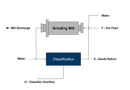
Circuit Figure 1
Where, (in dry tonnes ore per 24 hours)
F = New ore feed to grinding
M = Ore solids in mill discharge, or classifier feed
S = Coarse sands returned to mill
O = Classifier overflow product
And, liquid-to-solid dilution ratios of pulp samples
Dm = Mill discharge, or classifier feed if dilution water is added Ds = Classifier sands
Do = Classifier overflow
then the circulating load ratio
$R_{cl}= {CL \over F} = {D_o - D_m \over D_m - D_s}$
and, F x Rcl = CL, circulating load (tonnes/24 hours)
Or, if (F) is unknown:
Rcl x 100 = circulating load.
It will be seen from formula (21) that the capacity and separating efficiency of the classifier unit are critical factors governing the size of the circulating load, since CL becomes infinity where Dm equals Ds.
Example: A ball mill in closed circuit with a set of cyclones receives 1000 dry tonnes/day of crushed ore feed. The pulp densities for 0, M and S averaged 30, 55 and 72% respectively for an 8-hour shift, corresponding to D ratios of 2.33, 0.81 and 0.39. The circulating load ratio equals:
(2.33 - 0.81)/(0.81 - 0.39)=3.62 (362%)
and the circulating load tonnage is 3.62 x 1000 = 3620 tonnes/day.
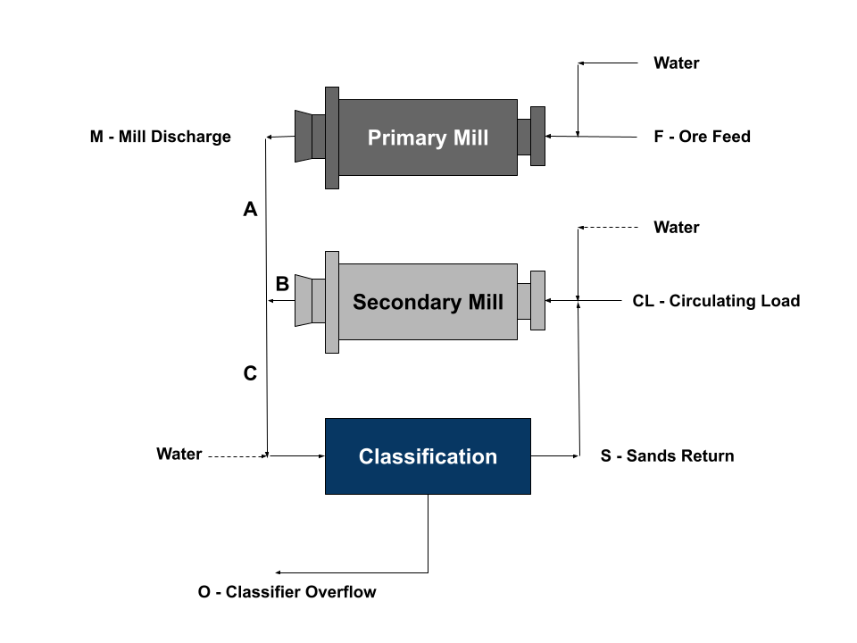
Circuit Figure 2
In this configuration another mill has been added to the previous circuit to increase grinding capacity. The new unit functions as the primary mill receiving only new ore feed (F), and operating in open circuit with the original mill which remains in closed circuit with the classifiers. The secondary mill now receives all of the circulating load, which can be estimated either by the previous method given, or by taking pulp samples A, B, and C to determine the respective dilution ratios, Da , Db , and Dc.
then,
$R_{cl} = {D_a - D_c \over D_c - D_d}$
Example: The product from a primary rod mill receiving 1500 tonnes/day of new ore feed joins the product of a secondary ball mill flowing to a sump feeding a set of cyclones in closed circuit with the ball mill. The pulp densities of samples taken at points A, B and C averaged 60, 71, and 67% solids respectively, equivalent to D ratios of 0.67, 0.41 and 0.49.
R_cl=(〖0.67〗_ - 0.49)/(0.49 - 0.41) =2.25 (or 225%)
CL=2.25×1500=3375 tonnes/day
Circulating loads based on screen analysis
A more precise method of determining grinding circuit tonnages employs the screen size distributions of the pulps instead of the dilution ratios. Pulp samples are screened and the cumulative weight percentage retained is calculated for several mesh sizes. The percentage through the smallest mesh can also be used to determine Rcl, as follows:
Figure 1: Circuit
Where,
m = Cum. wt. % on any mesh in the mill discharge, or classifier feed.
s = Cum. wt. % on the same mesh in the classifier sands.
o = Cum. wt. % on the same mesh in the classifier overflow.
Then,
$R_{cl} = {m - o \over s - m}$
Example: The same as circulating load using pulp densities where the screen analyses of the three samples are as follows.
Screen Analysis
Mesh Size | M | S | O | |||
% | Cum. % | % | Cum. % | % | Cum. % | |
+35 | 12.2 | - | 16.6 | - | - | - |
+48 | 27.1 | 39.3 | 34.7 | 51.3 | 0.8 | - |
+65 | 15.8 | 55.1 | 19.6 | 70.9 | 4.1 | 4.9 |
+100 | 10.3 | 65.4 | 9.6 | 80.5 | 12.8 | 17.7 |
+200 | 12.1 | 77.5 | 10.9 | 91.4 | 15 | 32.7 |
-200 | 22.5 |
| 8.6 |
| 67.3 |
|
Applying equation (23):
The + 65 mesh ratio =( 〖55.2〗_ - 4.9)/(70.9 - 55.2) = 3.18
The +100 mesh ratio =( 〖65.4〗_ = 17.7)/(80.5 - 65.4)= 3.16
The +200 mesh ratio =( 〖22.5 〗_ - 67.3)/(8.6 - 22.5)= 3.22
From the above, the average Rcl is 3.19. At a 1000 tonnes/day mill feed rate, the circulating load is 3190 tonnes per 24 hours.
Circuit Figure 2:
Where a, b, and c are the respective cumulative weight percentages for any given mesh size of samples A, B, and C, and F = New feed tonnage.
CL= Circulating load tonnage.
Then,
$a \cdot F+b \cdot CL=c \cdot(CL+F)$
then by rearrangement of equation 24a,
$R_{cl} = {CL \over F} = {a-c \over c-b}$
The calculations are then carried out in the same manner as for the previous example. It should be noted that errors in sampling and/or screen analyses may show widely divergent results on the different screen sizes. Any obvious anomalies should be discarded when averaging results.
Measuring an unknown tonnage by pulp dilution
If other procedures are not practical for determining the tonnage rate of solids flowing in a certain pulp stream, an approximate measurement may be obtainable using the pulp dilution method.
This procedure is based on adding a known amount of mill water to the pulp flow for which the tonnage estimate is needed, then determining the specific gravities and dilution ratios of the pulp before and after the water addition. Ore tonnage (F) is then estimated from:
$F = {L \over D_2-D_1}$
where, F= Tonnes per day dry ore in pulp
L = Tonnes per day mill water added
D2, and D1, are the dilution ratios in tonnes of water per tonne of ore, before and after the water addition, respectively.
Note: Chemical methods have also been suggested for determining unknown mill tonnage rates but such procedures are generally impractical for all but exceptional circumstances. If the reader is interested, reference5 listed at the end of this section covers the subject in detail.
7. Classifier and screen performance formulae
Classification efficiency is generally defined as the weight ratio of classified material in the sized overflow product to the total amount of classifiable material in the classifier feed, expressed as a percentage. For two-product separations, the general form used is:
$E = \text{% efficiency} ={O \over F} \cdot {(o-f) \over f(100-f)} \cdot 10,000$
Where,
F = Feed to Classifier, dry tonnes/day ore
O = Classifier overflow, dry tonnes/day ore
f = Wt. % of ore in feed finer than the mesh of separation (m.o.s.)
o = Wt. % of ore in the sized product finer than the m.o.s.
Example: Using the calculated tonnages and the screen analysis data from previous example, determine the classification efficiency of the cyclones at a m.o.s. of 65 mesh, where O = 1000, F = 4190, f = 44.9 and o = 95.1:
E=( 1000_ )/4190× ( 〖95.1-44.9〗_ )/((44.9)(100-44.9))×10,000=48.4% efficiency
Screening formulae
Where, a = Feed, wt.% coarser than m.o.s.
b = Feed, wt.% finer than m.o.s.
c = Oversize, wt.% coarser than m.o.s.
d = Oversize, wt.% finer than m.o.s.
f = Undersize, wt.% finer than m.o.s.
m.o.s. =Designated mesh of separation.
Recovery of undersize through the screen
$R = \text{wt. % recovery of fines} ={(c-a) \over (c+f)-100} \cdot 100$
Efficiency where undersize is desired product
$E_{screen} = \text{% screen efficiency} = {f \cdot R \over b}$
And for a quick estimate, E = 100 - d
Efficiency where oversize is desired product
$\text{100%}-R=O \text{, wt. % oversize}$
$E_{screen} = {c \times O \over a} \text{, % screen efficiency}$
Overall efficiency of screening
$E = {c \cdot O + f \cdot R \over 100} \text{, % overall efficiency}$
Concentration and recovery formulae
Using these formulae, the metallurgical performance of the concentration plant or of a particular mill circuit is readily assessed. They are similarly applied for calculating the results of laboratory testing. Since the computations are entirely dependent on the assays and weights, where known, of the process feed and products of separation, the calculated results are only as accurate as the sampling, assaying, and weighing methods employed to obtain the required data. As will also be seen, any increase in the number of separations and mineral components to be accounted for, greatly increases the complexity of the computations.
Two-product formulae
Applicable to the simplest separation where only one concentrate and one tailing result from a given ore feed.
Definition and Notation
Product | Weight or Wt. % | Sample Assay | Calculated |
Feed | F | f |
|
Concentrate | C | c |
|
Tailing | T | t |
|
Ratio of Concentration |
|
| K |
Recovery, % |
|
| R |
- Ratio of concentration can be thought of as the number of tonnes of feed required to produce one tonne of concentrate. The ratio, $\bar{K}$, for a separation can be obtained directly from the product weights or from the product assays if the weights are not known:
- $\bar{K} = {F \over C} = {c-t \over f-t} = \text{the concentration ratio}$
At operating plants, it is usually simpler to report the based on assays. If more than one mineral or metal is recovered in a bulk concentrate, each will have its own with the one regarded as most important being reported as the plant criteria. If the tonnage of concentrates produced is unknown it can be obtained using the product assays and the tons of plant feed:
$C= {F \over \bar{K}} = F\cdot({f-t \over c-t})$
Recovery, %
Represents the ratio of the weight of metal or mineral value recovered in the concentrate to 100% of the same constituent in the heads or feed to the process, expressed as a percentage. It may be calculated in several different ways, depending on the data available.
By assays f, c and t only:
$R = {c(f-t) \over f(c-t)} \cdot 100 = \text{% recovery}$
Using $\bar{K}$ plus assays f and c:
$R = {c \over f\cdot\bar{K}} \cdot 100 = \text{% recovery}$
By weights F and C, plus assays c and t
$R = 100 - {100\cdot t(F-C) \over c \cdot C + t(F-C)} = \text{% recovery}$
Example: A copper concentrator is milling 15,000 tonnes/day of a chalcopyrite ore assaying 1.15% copper. The concentrate and tailings produced average 32.7% and 0.18% copper, respectively. Calculate:
Per equation 31: $\bar{K}$=K=32.7-0.181.15-0.18=33.53
Per equation 32: C=15,000/33.53=447.4 tonnes
Per equation 33: R=((32.7)(1.15-0.18))/(1.15(32.7-0.18))×100=84.8%
Per equation 34: R=32.7/(33.53(1.15))×100=84.8%
8. Three-product (bi-metallic) formulae
Frequently, a concentrator will mill a complex ore requiring the production of two separate concentrates, each of which is enriched in a different metal or valuable mineral, plus a final tailing acceptably low in both constituents. Formulae have been developed which use the feed tonnage and assays of the two recovered values to obtain the ratios of concentration, the weights of the three products of separation, and the recoveries of the values in their respective concentrates. For illustrative purposes data from a copper-zinc separation is assumed.
Definition and Notation
Product | Weight or Wt.% | % Cu Assay | % Zn Assay | Calculated |
Feed | F | c1 | z1 |
|
Cu Concentrate | C | c2 | z2 |
|
Zn Concentrate | Z | c3 | z3 |
|
Tailing | T | c4 | z4 |
|
Ratios of Concentration |
|
|
| K |
Recovery, % |
|
|
| RCu and RZn |
The ratios of concentration, Kcu and Kzn are those for the copper and zinc concentrates, respectively, with Rcu and Rzn the percentage recoveries of the metals in their corresponding concentrates. As follows:
$C = F \cdot {(c_1-c_4)(z_3-z_4)-(z_1-z_4)(c_3-c_4) \over (c_2-c_4)(z_3-z_4)-(z_2-z_4)(c_3-c_4)} = \text{tonnes Cu concentrate}$
$Z = F \cdot {(c_2-c_4)(z_1-z_4)-(z_2-z_4)(c_1-c_4) \over (c_2-c_4)(z_3-z_4)-(z_2-z_4)(c_3-c_4)} = \text{tonnes Zn concentrate}$
$R_{Cu} = {c_2 \cdot C \over c_1 \cdot F} = \text{% copper recovery}$
$R_{Zn} = {z_3 \cdot Z \over z_1 \cdot F} = \text{% zinc recovery}$
$\bar{K}_{Cu}={F \over C}$ and $\bar{K}_{Zn}={F \over Z}$
Example:
Product | Tonnes | Cu | Zn |
Feed | 1000 | 2.7 | 19.3 |
Cu Concentrate | C | 25.3 | 5.1 |
Zn Concentrate | Z | 1.2 | 52.7 |
Tailings | T | 0.15 | 0.95 |
Then,
C = 1000 ×((2.7-0.15)(52.7-0.95)-(19.3-0.95)(1.2-0.15))/((25.3-0.15)(52.7-0.95)-(5.1-0.95)(1.2-0.15))
= 1000 ×(131.96-19.27)/(1301.51-4.36)=112.69/1297.15=86.9 tonnes of Cu concentrate
Z = 1000 ×((25.3-0.15)(19.3-0.95)-(5.1-0.95)(2.7-0.15))/((25.3-0.15)(52.7-0.95)-(5.1-0.95)(1.2-0.15))
= 1000 ×(461.50-10.58)/(1301.51-4.36)=450.9/1297.15=347.6 tonnes Zn concentrate
$R_{Cu}=((86.9)(25.3))/((1000)(2.7))×100=2198.6/2700×100=81.4%$
$R_{Zn}=((347.6)(52.7))/((1000)(19.3))×100=18318.5/19300.0×100=94.9%$
$〖\bar{K}_{Cu}=1000/86.9〗_ =11.51,\bar{K}_{Zn}=1000/347.6=2.88$
The three product solution illustrated above can be somewhat simplified by taking an intermediate tailings sample between the two stages of concentration i.e., a copper tail (zinc feed) sample in the previous example. Then, adding the notations:
Copper tail (zinc feed) = CT
with copper and zinc assays in said copper tails = c5 and z5, respectively. We assume mill feed F = 1.
Then, C + CT = 1
(C x c2)(CT x c5) = c1 (C x c3)(CT x c5) = c5
Subtracting (c) from (b),
C(c2–c5) = (c1–c5)
Then, C = F (c1–c5) = tonnes copper concentrate (c2–c5)
and similarly, Z = (F–C) (z5–z4) = tonnes zinc concentrate (z3–z4)
Example: It is decided to take a copper tail (zinc feed) sample in order to provide a check on the results calculated in the previous example. The sample (CT) assayed 0.55% Cu (c5) and 20.9% Zn (z5), respectively. The check weights of the copper and zinc concentrates are computed as follows:
Copper concentrate,
C=1000×((2.7-0.55))/((25.3-0.55))=1000×2.15/24.75=86.9 tonnes
Zinc concentrate,
Z=(1000-86.9)×((20.9-0.95))/((52.7-0.95))=913.1×19.95/51.75=352.0 tonnes
As can be seen, the calculated weights of the copper concentrate check exactly, while the zinc concentrate checks within 1.3%. An average of the zinc concentrate weights, obtained using both methods, could be used if desired.
It should be understood that there are certain limitations to the use of three-product formulae, since it is required by definition that two of the three products involved must be concentrates of essentially different metals or mineral components. The formulae will only give reliable results when the assays indicate that a differential concentration of the two components into separate concentrates has occurred.
9. Formulae for flotation reagent usage
The consumption or usage rate of the chemicals employed in flotation is generally expressed in terms of grams per metric ton of ore treated.
Depending upon the particular reagent, it may be fed as a dry solid, as a water solution or dispersion, or in the undiluted "as-is" liquid form. The normal procedure when checking or setting reagent feed rates is to measure the amount being fed to the circuit per unit time, usually per minute. Liquid or reagents in solution or dispersion are measured in ml and dry solids in grams. When feeding liquids, the specific gravity and weight percent strength of the reagent must also be known. With this information, along with the known ore tonnage being treated per unit time, the reagent measurements can then be translated into grams/metric ton consumption rates, as follows:
For dry reagents
${\text{(g reagent/min)(1440 min/day)} \over \text{tonnes ore/day}} = {\text{g reagent} \over \text{tonne ore}}$
For liquid reagents
${\text{(ml reagent/min)(reagent sp. gravity)(1440 min/day)} \over \text{tonnes ore/day}} = {\text{g reagent} \over \text{tonne ore}}$
For reagents in solution
${\text{(ml reagent/min)(g reagent/liter solution)(1440 min/day)} \over \text{tonnes ore/day}} = {\text{g reagent} \over \text{tonne ore}}$
Example: At a 10,000 tonnes/day milling rate, a plant is using 590 ml/min. of a 200 g/L xanthate solution. Calculate the dosage rate.
((590)(200)(1440))/(10000×1000)=17 g/t
10. Material balance software
Material balance software for mineral processing flowsheets have been available for over 50 years since the development of MATBAL by Wiegel in 1970. These material balance software programs are capable of calculating coherent, multicomponent mass balances based only upon assays and measured flow rates. The objective of the mass balance is to determine the weight (mass) for each of the process streams in a circuit. Since the weights of streams in a mineral processing flowsheet are quite large, most streams are left unmeasured. At most operations there is often only one measured flow rate, the feed, with the rest of the process streams weights being unknown. Therefore the mineral processor must rely upon assays of each process stream in order to calculate a coherent, multicomponent mass balance. Since the assays and any available weights are only estimates of the true value, the material balance is accomplished by adjusting the estimates of the assays and the weights of all flows until all of the laws of conservation of mass are met. In most mass balance situations there are usually more equations than there are unknown values, which is an overdetermined system. Therefore, there is no exact solution. There is theoretically an infinite number of solutions. A solution can be found by minimizing the sum of the squares of all the adjustments of the observed assays and weights. A search routine can be used to determine the minimum.
The laws of conservation of mass for a mineral processing circuit are met when the weights (W) of each stream entering and leaving the circuit sum to zero for any one node in the circuit (Type 1) and the product of the weight and the assay (W⋅X) for each stream entering or leaving the circuit sum to zero (Type 2) as shown below.
$Type 1: W1-W-W3 = 0$
$Type 2: W1\cdot X1-W2\cdot X2-W3\cdot X3 = 0$
There are a few commercially available computer software packages available for the computation of coherent, multicomponent mass balances of mineral processing circuits. Two of the commercially available software programs include Bilmat™ from Triple Point Technology and JKMultiBal from JKTech Pty Ltd. The mineral processor could also use the Solver add-in of Microsoft® Excel® to arrive at a coherent, multicomponent mass balance.
An example of the use of the Solver add-in of Microsoft® Excel® for the calculation of a material balance for a mineral processing flowsheet is described below.
Example:
A large copper-zinc operation produces a copper concentrate, a zinc concentrate, and a final tailings and from mill feed. The assays and weight (flow rate) of an internal stream, the copper circuit tailings or zinc circuit feed, is needed in order for the flotation operator to know the performance of the copper circuit and also to set the addition rate for copper sulfate addition for the zinc flotation circuit. Copper, zinc, and iron assays are available for each of the 5 process streams and are shown in Table 2. Figure 3 illustrates a simplified flowsheet for the operation’s flotation plant.
Stream | Weight (tph) | Observed Assays (%) | |||
# | Name | Observed | Cu | Zn | Fe |
1 | Feed | 100 | 1.69 | 4.6 | 17.5 |
2 | Cu Conc | n/a | 20.9 | 6.0 | 28.6 |
3 | Cu Tails | n/a | 0.2 | 4.3 | 16.6 |
4 | Zn Conc | n/a | 1.05 | 52 | 10.7 |
5 | Final Tails | n/a | 0.09 | 0.52 | 17.0 |
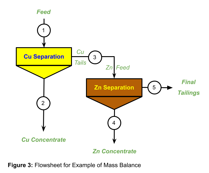
In order to calculate a mass balance using the generalized least squares methodology, the calculations are usually accomplished in two steps. The first step requires providing initial weight estimate values and the second step completes the calculation using these initial weight estimates. Any search routine, including Solver, requires a reasonable set of initial values to narrow the search space to avoid localized minimums, trivial solutions (all zeros), and nonsensical (negative) results. The minimization of node imbalances methodology provides better initial weight estimates, when working with several assays (components), than averages of several n-product formulae or regressions. Once the initial weight estimates are determined, a coherent balance can then be calculated using generalized least-squares methodology.
Step 1: Minimization of Node Imbalances (constrained)
A constrained node imbalance procedure assumes that weights (W) for each node follow the law of conservation of mass (Type 1) as can be seen in the constraints listed below. However, at this point the observed (measured) values of the assays are considered the best estimates. In other words there is no adjustment of the observed assays for this step. Since there is no adjustment of the observed assays, none of the Type 2 equations will be satisfied and there will be imbalances for each node and each assay.
Constraints:
$W_{obs}^1=W_0^1=100$, alternatively this could be added as an imbalance $(W_0^1-W_{obs}^1)\over \sigma$ instead of as a constraint. A very small standard deviation would effectively set the initial weight to the observed weight.
$W_0^1-W_0^2-W_0^3=0$
$W_0^3-W_0^4-W_0^5 =0$
Imbalances:
$W_0^1\cdot X1_{obs}^{Cu}-W_0^2 \cdot X2_{obs}^{Cu} - W_0^3\cdot X3_{obs}^{Cu} = I_1^{Cu}$
$W_0^1\cdot X1_{obs}^{Zn}-W_0^2 \cdot X2_{obs}^{Zn} - W_0^3\cdot X3_{obs}^{Zn} = I_1^{Zn}$
$W_0^1\cdot X1_{obs}^{Fe}-W_0^2 \cdot X2_{obs}^{Fe} - W_0^3\cdot X3_{obs}^{Fe} = I_1^{Fe}$
$W_0^3\cdot X1_{obs}^{Cu}-W_0^4 \cdot X2_{obs}^{Cu} - W_0^5\cdot X3_{obs}^{Cu} = I_2^{Cu}$
$W_0^3\cdot X1_{obs}^{Zn}-W_0^4 \cdot X2_{obs}^{Zn} - W_0^5\cdot X3_{obs}^{Zn} = I_2^{Zn}$
$W_0^3\cdot X1_{obs}^{Fe}-W_0^4 \cdot X2_{obs}^{Fe} - W_0^5\cdot X3_{obs}^{Fe} = I_2^{Fe}$
Then minimize the sum of the squares of all of the imbalances listed above
$(I_1^{Cu})^2+(I_1^{Zn})^2+(I_1^{Fe})^2+(I_2^{Cu})^2+(I_2^{Zn})^2+(I_2^{Fe})^2 = minimum$
Where:
$W_{obs}^1 = \text{Observed weight estimate of stream 1}$
$W_0^n = \text{Initial weight estimate of stream n}$
$Xn_{obs}^b = \text{Observed component assay for stream n and component b}$
$I_m^b = \text{Node imbalance for node m and component b}$
You can watch an instructional video below to learn how to complete the minimization of node imbalance portion of the mass balance calculations.

| Weights | Observed Assays (%) | Adjusted Assays (%) | ||||||
Stream # | WObs. | W0 | Wadj | Cu | Zn | Fe | Cu | Zn | Fe |
1 | 100 | 100.00 |
| 1.69 | 4.6 | 17.5 |
|
|
|
2 | n/a | 7.33 |
| 20.9 | 6 | 28.6 |
|
|
|
3 | n/a | 92.67 |
| 0.2 | 4.3 | 16.6 |
|
|
|
4 | n/a | 6.79 |
| 1.05 | 52 | 10.7 |
|
|
|
5 | n/a | 85.88 |
| 0.09 | 0.52 | 17 |
|
|
|
Step 2:
Now that the initial weights for each of the streams have been determined the calculations can proceed to Step 2. While completing this portion of the calculation all of the Type 1 and Type 2 constraints can be used. The feed weight can also be constrained to a value of 100.
Constraints:
$W_{obs}^1=W_0^1=W_{adj}^1=100$
| Node 1 | Node 2 |
Type 1 | $W_{adj}^1-W_{adj}^2-W_{adj}^3 = 0$ | $W_{adj}^3-W_{adj}^4-W_{adj}^5 = 0$ |
Type 2 | $W_{adj}^1\cdot X1_{adj}^{Cu}-W_{adj}^2\cdot X2_{adj}^{Cu}-W_{adj}^3\cdot X3_{adj}^{Cu}=0$ | $W_{adj}^3\cdot X3_{adj}^{Cu}-W_{adj}^4\cdot X4_{adj}^{Cu}-W_{adj}^5\cdot X5_{adj}^{Cu}=0$ |
| $W_{adj}^1\cdot X1_{adj}^{Zn}-W_{adj}^2\cdot X2_{adj}^{Zn}-W_{adj}^3\cdot X3_{adj}^{Zn}=0$ | $W_{adj}^3\cdot X3_{adj}^{Zn}-W_{adj}^4\cdot X4_{adj}^{Zn}-W_{adj}^5\cdot X5_{adj}^{Zn}=0$ | |
| $W_{adj}^1\cdot X1_{adj}^{Fe}-W_{adj}^2\cdot X2_{adj}^{Fe}-W_{adj}^3\cdot X3_{adj}^{Fe}=0$ | $W_{adj}^3\cdot X3_{adj}^{Zn}-W_{adj}^4\cdot X4_{adj}^{Zn}-W_{adj}^5\cdot X5_{adj}^{Zn}=0$ |
Minimizing:
At this point it is desirable to have the observed assays adjusted as little as possible in order to achieve a coherent mass balance. Therefore the objective now becomes minimization of the sum of the squares of the residuals (X_obs-X_adj) for all of the assays (components).
$\sum (X_{obs}-X_{adj})^2 = \text{minimum}$
Mineral processing circuits usually have some observed weights or assays which are considered more reliable than others. It may be desirable to weight the more reliable data more heavily in the mass balance calculations. Weighting each variable adjustment using the reciprocal of the variance for any one assay or weight is an appropriate method. By using the reciprocal of the variance it can be appreciated that a smaller variance will result in greater weighting and conversely a larger variance will result in lesser weighting.
$\sum {(X_{obs}-X_{adj})^2 \over \sigma^2} = \text{minimum (weighted sum of the square of residuals)}$
${(X1_{obs}^{Cu}-X1_{adj}^{Cu})^2 \over (\sigma_1^{Cu})^2}+{(X2_{obs}^{Cu}-X2_{adj}^{Cu})^2 \over (\sigma_2^{Cu})^2}+{(X3_{obs}^{Cu}-X3_{adj}^{Cu})^2 \over (\sigma_3^{Cu})^2}+{(X4_{obs}^{Cu}-X4_{adj}^{Cu})^2 \over (\sigma_4^{Cu})^2}+{(X5_{obs}^{Cu}-X5_{adj}^{Cu})^2 \over (\sigma_5^{Cu})^2}=\sum {(Xn_{obs}^{Cu}-Xn_{adj}^{Cu})^2 \over (\sigma_n^{Cu})^2}$
${(X1_{obs}^{Zn}-X1_{adj}^{Zn})^2 \over (\sigma_1^{Zn})^2}+{(X2_{obs}^{Zn}-X2_{adj}^{Zn})^2 \over (\sigma_2^{Zn})^2}+{(X3_{obs}^{Zn}-X3_{adj}^{Zn})^2 \over (\sigma_3^{Zn})^2}+{(X4_{obs}^{Zn}-X4_{adj}^{Zn})^2 \over (\sigma_4^{Zn})^2}+{(X5_{obs}^{Zn}-X5_{adj}^{Zn})^2 \over (\sigma_5^{Zn})^2}=\sum {(Xn_{obs}^{Zn}-Xn_{adj}^{Zn})^2 \over (\sigma_n^{Zn})^2}$
${(X1_{obs}^{Fe}-X1_{adj}^{Fe})^2 \over (\sigma_1^{Fe})^2}+{(X2_{obs}^{Fe}-X2_{adj}^{Fe})^2 \over (\sigma_2^{Fe})^2}+{(X3_{obs}^{Fe}-X3_{adj}^{Fe})^2 \over (\sigma_3^{Fe})^2}+{(X4_{obs}^{Fe}-X4_{adj}^{Fe})^2 \over (\sigma_4^{Fe})^2}+{(X5_{obs}^{Fe}-X5_{adj}^{Fe})^2 \over (\sigma_5^{Fe})^2}=\sum {(Xn_{obs}^{Fe}-Xn_{adj}^{Fe})^2 \over (\sigma_n^{Fe})^2}$
Where:
$W_{adj}^n=\text{Adjusted weight of stream n}$
$Xn_{obs}^b=\text{Observed component assay for stream n and component b}$
$Xn_{adj}^b=\text{Adjusted component assay for stream n and component b}$
$(\sigma_n^b)^2=\text{Variance for stream n and component b}$
You can watch an instructional video below to learn how to complete the generalized least square (GLS) portion of the mass balance calculations.

The results after completion of the mass balance calculations are shown in Table 5 and Table 6 . No weighting of the assays (components) was used to arrive at the results in Table 5. A weighting of 5% relative standard deviation was used to arrive at the results in Table 6.
| Weights | Observed Assays (%) | Adjusted Assays (%) | ||||||
Stream # | WObs. | W0 | Wadj | Cu | Zn | Fe | Cu | Zn | Fe |
1 | 100 | 100.00 | 100 | 1.69 | 4.6 | 17.5 | 1.71 | 4.50 | 17.47 |
2 | n/a | 7.33 | 7.46 | 20.9 | 6 | 28.6 | 20.90 | 6.01 | 28.60 |
3 | n/a | 92.67 | 92.54 | 0.2 | 4.3 | 16.6 | 0.17 | 4.38 | 16.57 |
4 | n/a | 6.79 | 6.93 | 1.05 | 52 | 10.7 | 1.05 | 52.00 | 10.70 |
5 | n/a | 85.88 | 85.61 | 0.09 | 0.52 | 17 | 0.10 | 0.53 | 17.05 |
| Weights | Observed Assays (%) | Adjusted Assays (%) | ||||||
Stream # | WObs. | W0 | Wadj | Cu | Zn | Fe | Cu | Zn | Fe |
1 | 100 | 100.00 | 100 | 1.69 | 4.6 | 17.5 | 1.69 | 4.62 | 17.44 |
2 | n/a | 7.33 | 7.30 | 20.9 | 6 | 28.6 | 20.90 | 6.00 | 28.61 |
3 | n/a | 92.67 | 92.70 | 0.2 | 4.3 | 16.6 | 0.18 | 4.51 | 16.56 |
4 | n/a | 6.79 | 7.57 | 1.05 | 52 | 10.7 | 1.10 | 49.36 | 10.70 |
5 | n/a | 85.88 | 85.12 | 0.09 | 0.52 | 17 | 0.09 | 0.52 | 17.08 |
11.Bibliography and References
- The Denver Equipment Co., Handbook, 1954 Edition.
- Mineral Processing Flowsheets:Denver Equipment Co., Denver, CO, 1962.
- Taggart, A. F., Handbook of Mineral Dressing, J. Wiley & Sons, Inc., New York, 1945.
- Weinig, A. and Carpenter, C., The Trends of Flotation, Colorado School of Mines Quarterly, Vol. 32, No. 4, October, 1937.
- Williamson, D. R., The Mathematics of Concentration Processes, Colorado School of Mines Mineral Industries Bulletin, Vol. 3, No. 6, November, 1960.
- Kelly, E.G., and Spottiswood, D.J, Introduction to Mineral Processing; John Wiley & Sons Inc., New York, N.Y., 1982.
- Weiss, N.L., SME Mineral Processing Handbook; Society of Mining Engineers, New York, N.Y., 1985.
- Wills, B.A., Mineral Processing Technology; ButterworthHeinemann, Oxford, UK, Sixth Edition, 1997.
- Yianatos, J.B., and Henríquez, F.D., Minerals Engineering, Vol. 19, Issue 13, Nov. 2006, p-1336-1340.
- Cortes et al., Copper 95', Mineral Processing & Environment, Vol.
- R.L. Wiegel (1972) Advances in mineral processing material balances, Canadian Metallurgical Quarterly, 11:2, 413-424, https://doi.org/10.1179/cmq.1972.11.2.413