
Introduction
Laboratory flotation testing can be a time-consuming and costly process. The need to produce quality results and formulate relatively accurate and concise conclusions from the resources invested is vitally important. Hence, a systematic investigation using good experimental techniques and consistent laboratory testing procedures must be followed. The information presented here is not meant to be exhaustive and should be used only as a guideline. Careful thought should be given before undertaking any type of large-scale testing. Experience and intuition play an important role in developing testing protocols and a useful experimental design to answer these questions. An understanding of the types of variation (ore to ore, flotation operator to operator, assay variations etc.) and their effect is important in flotation test work in order to obtain meaningful results. For example an operator may conduct three flotation tests under the same exact conditions and may still get three different answers. Or two different operators may conduct the same flotation test and also get different answers between them. The message here is that there is inherent variability in laboratory flotation testing and the testing program should be designed to address this variation so that one can have confidence in the results obtained. FLOTATION MATRIXTM 100 methodology, is the recommended approach to address these issues and provide a robust and optimized laboratory test program to match the specific process needs.
The following guidelines are discussed in this section:
- Sampling for laboratory flotation – ideally should be representative of normal plant feed. It would also be of benefit to obtain different ore types from different sections of the mine to map flotation performance or to generate a more robust solution to address the various ore types that a concentrator may encounter.
- Microscopic analysis (reflected light microscopy, QEM-SEM, MLA) – to determine mineralogy, morphology, mineralogical associations and degree of liberation. Oftentimes these tools will aid the metallurgist in determining if the ore is even amenable to beneficiation using present-day separations techniques.
- Ore preparation – Representative sub-sampling and handling of ore for laboratory flotation testing to ensure that each test contains the equivalent minerals or metals content.
- Grinding – to achieve the desired degree of liberation of value minerals.
- Test design – provide a framework of desired tests to answer a particular question(s) or to formulate an ore treatment solution. The objectives should be clear and concise with measurable metrics.
- Laboratory flotation – tool for screening of reagents and other variables for improved metallurgical performance, but is not meant to optimize concentrator performance which is better handled at the plant scale.
- Handling of flotation products filtration, drying, packaging for analysis.
- Assaying – to determine separations efficiency and generate mass balances to evaluate overall flotation performance.
- Data analysis/Interpretation of results – statistical vs. traditional empirical approach to determine if the objectives have been met or the initial question(s) has been answered. Did we accomplish what we set out to do; did we answer all our questions? May also provide direction for any additional tests that may be required.
Ore Sampling for Laboratory Flotation
When ore samples are taken directly from the belt feed or stockpile, it should be borne in mind that no two ore bodies are the same, and that variations within an ore body are common. These variations would include mineral speciation and their various associations, degree of dissemination, locking of sulfides with each other and with non-sulfide gangue minerals, degree of alteration due to tarnishing or oxidation, etc. Close consultation with the milling, mining and geology departments is essential in determining the proper selection of an ore sample(s) for testing. The various ore types chosen will also be highly dependent on the objectives of the project.
Generally, the amount of ore for laboratory test work should be sufficiently large so that an entire investigation or 2-3 blocks of well designed tests can be completed on one sample without having to re-sample the deposit. If re-sampling becomes necessary then one should be aware of the possibility of new sources of variation being introduced into your analysis. It is often better to have more ore than necessary rather than not enough. Designing the test program and determining the number of tests needed ahead of time will help you determine how much ore to prepare.
In the case of concentrators in operation, ore samples may be taken from the conveyor belt feeding coarse ore to the grinding section (i.e., SAG or rod mill feed). Samples should also be taken over a sufficient period of time so that the ore will be representative of current mill feed (run-of-mine or ROM). One should also bear in mind that this represents just a "snapshot" in time from a specific location within the mine or pit. If the objectives warrant, additional ore sampling can be taken from various locations within the mine or pit to map the performance of the various ore types, or to develop a more robust solution for the varying ore types. The latter is the basis for the FLOTATION MATRIXTM 100 process.
The collected ore should be labeled with the name of the mine owner, the name of the mine or concentrator, the name of the specific type of ore or its location in the pit, date of retrieval, and any other special ore characteristics that would clearly differentiate the ore from other ores. If the ore is to be shipped to another location, the paperwork and container(s) should be clearly marked with the above identification.
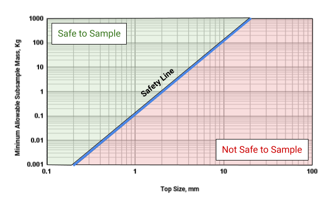
One important thing to keep in mind is the required mass of ore needed to obtain a truly representative sample. Based on Pierre Gy’s theory of sampling, a safety line of sampling based on particle top size has been defined as shown in Figure 1. The safety [sampling] line represents the minimum allowable subsample mass that will be representative of the original mass. Two regions are defined: To the left of the safety line is the safety zone where any combination of particle top size and subsample mass is representative of the sampled mass; to the right is the zone in which any combination of top size and subsample mass will not be representative of the sampled mass. This applies to all sampling aspects including splitting charges for flotation and sub-sampling lab flotation products for assaying or mineralogical analysis.
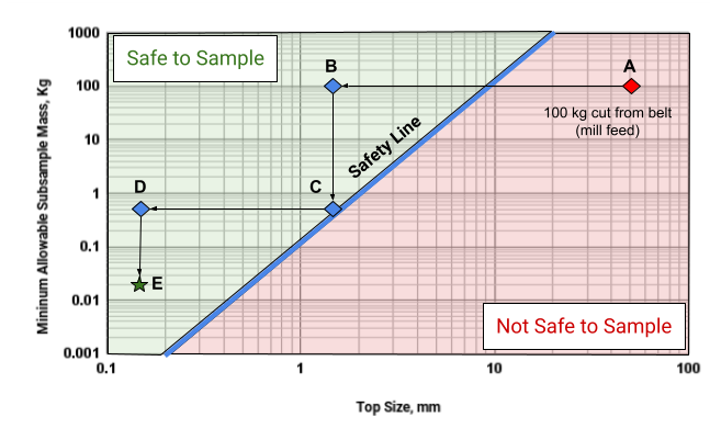
For example, as shown in Figure 2, a belt cut is made in order to obtain about 100 kg with a 50 mm top size (point “A”). Note that this places this particular subsample (of the stockpile) in the “Not Safe to Sample” zone, however, this will have to do given that, obtaining a truly representative sample at this point would require one to collect > 1000 kg of material, which although achievable, may not be practical. Our first step is to split this material into representative (equal) charges for flotation. Therefore, the first step is to stage-crush the material (by multiple rounds of jaw-, cone-, roll crushing, and 10 mesh sieving) to a top size of approximately 2 mm (10 mesh), leaving us at point “B”. We are now able to split the material into 200 charges of 500 g each (point “C”). During our test program, for a single test we grind a charge to a top size of 150 microns (point “D”). After filtering and drying of the test’s flotation products, approximately 20 g each of tails and concentrates are sent for assaying (point “E”).
For a copy of a printable safety line sheet please click HERE.
When taking pulp samples, it is advisable to verify that the plant is operating under normal conditions. Gross deficiencies in grinding or cyclone operation could lead to collection of a pulp sample with the incorrect granulometry. Temporary changes in feed, with respect to ore type different from ROM, can lead to erroneous conclusions from conducting tests on the wrong ore.
It is recommended that fresh pulp samples be taken daily, since ground ore is subject to aging effects more rapidly than the uncrushed ore. It is further suggested that sufficient pulp sample be taken in the morning or in the afternoon, just prior to flotation testing to help reduce the effect of pulp aging. Enough pulp should be collected to conduct a block of 4-6 tests before additional pulp is collected. If all of the pulp required for a testing program is collected all at once (i.e. for 8-12 tests), one should note that the pulp tested at the very beginning will be different from the pulp tested at the end, due to aging effects. In this case it may be useful to conduct control tests in the beginning and the end of the program and randomize the runs as explained in the Statistical Methods in Minerals Processing section. In addition, the pulp should also be free of any collectors or modifiers that may interfere with your evaluation. If necessary, request that any reagent dosing be temporarily turned off upstream of the collection point. For convenience and if easily accessible, it may be desirable to take classifier/cyclone overflow pulp, so that flotation feed size distribution is the same as that of the concentrator/plant. The pulp samples should be labeled with the date, time of day and circuit location where the sample was taken.
Microscopy
Microscopical examination of the feed samples is highly desirable to identify minerals present in the ore and to determine mineral textures and associations with other minerals. The availability of this information can assist in the design of the test program and reagent selection. You may also obtain this information from the plant Metallurgists, Geologists, Mineralogists or Microscopists.
The feed samples should be examined by a qualified microscopist/mineralogist, using the appropriate techniques such as reflected light microscopy, Quantitative Electron Microscopy – Scanning Electron Microscopy (QEM-SEM), Mineral Liberation Analyzer (MLA) and X-Ray Diffraction, powder (XRD).
The proper use of the aforementioned techniques can also be a valuable "trouble-shooting" tool to aid in determining the types of minerals being recovered in the concentrate, as well as what is being lost in the tail (rejects) when a particular reagent scheme is used. Oftentimes these techniques will aid in determining if the ore is economically amenable to flotation.
Please refer to the relevant section “Applied Mineralogy and Mineral Surface Analysis” for further discussion.
Ore preparation
Dry ore
The dried ore sample must be transported to the test laboratory as quickly as possible, preferably in a coarse state (1-2 cm) to keep oxidation to a minimum. The sample is then typically stage-crushed to minus 1-2 mm (10 Tyler mesh), for ease of splitting, packaging and grinding. The ore can be blended thoroughly, using a riffler or rotary splitter. The ore is then converted to flotation charges of the desired weight with a rotary splitter to ensure that the metal/mineral content is equivalent from charge to charge. The ore charges should then be sealed in plastic bags, labeled with the name of the mine owner, concentrator, specific type of ore or its location in the pit, date of retrieval, and any other special ore characteristics that would clearly differentiate the ore from other ores, and stored in a freezer (preferably -15°C or lower) to retard oxidation/aging effects. Several randomly chosen charges should be submitted for head grade analysis to confirm that the sample splitting has been conducted correctly, and that the charges contain equivalent metal content.
Pulp samples
The amount of pulp sample taken at any one time is dependent on many factors. These include:
- Percent solids of the pulp
- The size of the laboratory flotation cell
- The number of flotation tests to be conducted in a particular series; and,
- The degree to which the pulp is known to be sensitive to aging effects.
Sub-sampling of the pulp into flotation charges can be done either volumetrically or, preferably, gravimetrically while the pulp is being adequately agitated. When the situation is such that the pulp has to be used for an extended test series, then test charges should be placed in sealed containers and stored in a freezer. The charges are prepared by agitating the pulp to keep the solids suspended; a portion of the pulp should be collected using a ladle or beaker and alternately placed into one of however many jars of pulp may be required for the subsequent testing. The procedure continues alternately, placing portions of pulp into each jar before returning to the first jar, until all the jars are full or the pulp sample is consumed. Note that the jars should be of sufficient size to allow for a 2-3 cm headspace when filled with pulp to accommodate the expansion of the pulp as it freezes. When needed for testing, the pulp is thawed first and transferred, if necessary, from one or more jars directly into the flotation cell.
Sampling may also be conducted with a rotary slurry/pulp sampler available from some equipment suppliers to the mining industry.
Grinding
Laboratory grinding tests are conducted primarily to establish the size distribution of the solids and adequacy of liberation of the value minerals which is dictated by the objectives of the test work.
Mesh of liberation
This is estimated by examining various screen size fractions of the ground ore (usually the coarser fractions) using reflected light microscopy. This provides information on the modes of occurrence and the degree of liberation of the desired minerals, i.e., sulfide-gangue mineral associations.
If a microscopical facility or expertise is not available, the optimum liberation size can be estimated by a granulometry vs. flotation recovery curve.
Granulometry versus grinding time relationship
By graphically plotting the cumulative weight percent passing (or retained on) a screen size vs. the log grinding time, a relatively straight line will result between about 15% and 85% cumulative weight for that screen size. It is then a simple matter to change the grinding times during the test program in order to change the flotation feed granulometry. Occasionally one may find coarse ground material
Experience at Syensqo favors the use of a rod mill for laboratory batch grinding as opposed to a ball mill, to minimize formation of slimes/ultrafines. The pulp density for grinding is generally in the range of 60% to 70% solids, depending on the ore's pulp viscosity and the specific gravity of the dry solids.
The ground pulp should be wet screened on a 200 mesh (74 µm) or 325 mesh (44 µm) sieve and the oversize and undersize (slimes) material filtered and dried separately. The oversize is then dry-screened on a series of sieves, generally from about 500 µm through 74 µm or 44 µm (depending on the original size used for the wet screening). Any material passing through the finest sieve should be added to the undersize from the wet screening operation. The weights of the various screen fractions are then used to determine the size distribution of the ground ore. Stainless steel sieves are recommended for most routine screening. The procedure noted above can be conducted on a 200 gram aliquot from the larger ground ore sample to avoid excessive retention of ore on the screens which can cause "blinding".
Test Design
Prior to undertaking any extensive reagent testing program, the objectives for such a program should be clearly defined. The variables or factors (i.e. ore type, collector type, collector dosage, frother type, frother dose, pH, etc.) to be studied should be well thought out, along with the levels of treatment to use in order to observe the desired response and to determine the relative importance of these variables. A thorough investigation of all of the variables involved in a process is not practical. The variables selected for study will depend on the objectives of the investigation, as well as feedback from observations and results (if available) from preliminary diagnostic tests used to set testing levels (i.e. 20 g/t vs. 30 g/t or pH 9 vs. pH 11). Variables not under investigation should be kept as constant as possible.
An often used approach of changing one factor at a time (OFAT) has serious limitations, as will be described in Statistical Methods in Mineral Processing. It is highly recommended that an experimental design or DOE (Design of Experiments) based on statistical principles be performed, which will enable the researcher to investigate the effects of several variables simultaneously. Carefully planned experiments conducted in this manner will provide more information than the OFAT approach with a fewer number of tests.
There are many references to statistical experimental designs in the literature. Syensqo's representatives have been appropriately trained in developing experimental designs and can assist the customer in this respect.
Flotation Testing
In designing a flotation test program, experience plays an important role in minimizing the number of variables and the range over which these variables need to be tested. Knowledge of how other concentrators are treating similar ores is a valuable tool for the metallurgist. Syensqo personnel offer this experience and knowledge, as a result of metallurgical investigations conducted at many plants and with many ores from around the world.
Grind-granulometry
The grinding range to be evaluated will be largely influenced by the microscopical examination of various screen fractions, referred to previously. Because of the operating costs associated with grinding, a common plant practice is to grind as coarsely as possible, without sacrificing rougher recovery; the rougher concentrate then requires regrinding for adequate mineral liberation, prior to cleaner flotation. Evaluation of regrinding should be conducted using the information presented in the Grinding section. Proper selection of collector combinations may allow utilization of a coarser grind without loss of rougher recovery.
In the case of complex ores, where recovery of two or more mineral values into separate concentrates is desired, coarse primary grinding may not be practical. Due to the resulting complex regrinding and cleaning circuits, with large and sometimes unstable circulating loads, circuit control on a plant scale may not be manageable. In such cases, it may be preferable to grind finer for adequate mineral liberation ahead of the rougher stage, thereby simplifying circuit design and control.
We recommend cleaning the laboratory mill by grinding coarse quartz silica (200-500 g), prior to each day's testing, to remove rust and residual reagents. It is also good practice to condition the mill with the pH modifier at this time by adding the pH modifier during the mill cleaning stage.
Due to the natural plant variability in granulometry, it is recommended that granulometry or grind time be included as a variable in any laboratory experimental design. The range of operation for the mill can be obtained from the plant metallurgists.
Conditioning and points of reagent addition
The conditioning time and reagent addition points can have a large influence on metallurgy, particularly under plant operating conditions. For plants currently in operation, the reagent points-of-addition and conditioning times should be adhered to for the standard or control test, but one should also bear in mind that changing the reagent addition points and split addition could produce better metallurgy and should be included in any experimental test design. The effect of collector stage-addition or split addition and the use of different collectors at varying points in the proposed circuit should also be evaluated. For example, oily collectors are generally, but not always, added in the grinding circuit. These collectors can also be added to cyclone overflow or conditioning box as long as there is sufficient turbulence to adequately disperse the reagent.
Addition points of frothers, activators and modifiers can vary, depending on the mineral associations, water quality and types of collector being evaluated. Optimum points of addition for these reagents usually become more apparent from visual observations, and after conducting some preliminary diagnostic tests and evaluating the metallurgical results.
We recommend adding the reagents using a syringe, microliter syringe or pipette of sufficient volume, depending on the reagent concentration and dosages required. Water soluble reagents may also be further diluted to achieve the desired dosing requirements. Dilution of oily collectors for laboratory testing is not straightforward and is highly dependent on the chemistry of the collector. Normally a solvent is chosen that exhibits neutral metallurgical performance, unless the desire is to enhance synergistic effects by using a frother as a diluent. Contact a Syensqo representative before undertaking any such dilution, as they can also address any safety related issues. Never mix any chemicals together without first consulting the Safety Data Sheets, Technical Data Sheets or a Syensqo representative.
pH and alkalinity
The usual practice is to float at natural pH or in an alkaline circuit, adjusted with lime (calcium hydroxide) or milk of lime. In some cases, the use of soda ash (sodium carbonate), sodium hydroxide or ammonia may have an advantage. Acid circuits are utilized if the metallurgical advantages outweigh the higher equipment and operating costs. pH adjustment is best made in the grinding mill with minor adjustments in the flotation cell. The amount of pH modifier to add is usually based on trial and error, and once established should remain constant for all the tests, unless it is a variable under investigation. The recovery vs. pH of certain minerals is documented in the literature. Typical pH operating ranges for various ore types are discussed under separate headings for those ores.
Because pH cannot be precisely maintained in the plant, it is recommended that pH be included as a variable in any laboratory experimental design. The range of operation for the mill can be obtained from the plant metallurgists. There may also be an opportunity to operate at a lower pH, thereby reducing pH modifier consumption with the optimum choice of reagents. This opportunity can only be explored if pH is included in a DOE.
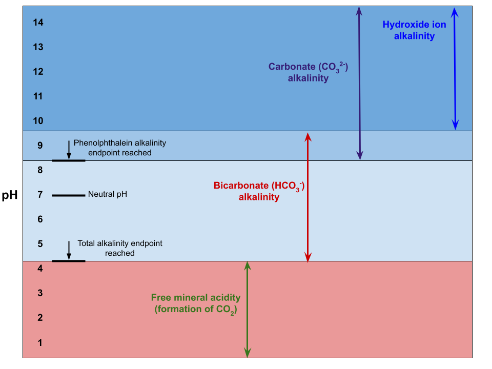
Alkalinity measures the ability of a given aqueous sample to neutralize acid. It is important to recognize that pH and alkalinity are not the same thing. pH is a measure of intensity (or concentration) of H+ per definition. Alkalinity, on the other hand, aside from hydroxide ions, also takes into account the contribution of other acid-neutralizing ions, mainly from carbonate (CO32-) and bicarbonate (HCO3-) ions and is thus a measure of capacity. Note that there are other species that can contribute to alkalinity including but not limited to phosphates, silicates, borates, hydrosulfide (HS-), ammonia, organic ligands (e.g. acetate, propionate) and, of course, hydroxide ion; the contribution of hydroxide ion only becomes significant at pH > 10. Alkalinity is a better indicator of changes in acid-neutralizing capacity above pH of 11.5, where pH is significantly less sensitive; below this pH value, particularly below pH 11, measuring pH is a better indicator of changes in acid-neutralizing capacity, say, from addition of lime. Alkalinity at these lower pHs is not a good substitute for pH, given that there can be large variability in pH at a given alkalinity. It is also important to note that measuring alkalinity of the slurry and not of a filtrate or supernatant of the slurry would be more appropriate given that many minerals (e.g. carbonates) undergo reactions with protons in solution, and thus contribute to the total alkalinity. However, measurements on slurry tend to be erratic and measurement of alkalinity on supernatant or filtrate is more routinely encountered.
Although pH and alkalinity are not directly related, measurements of alkalinity by titration do use pH as an end-point value for interpretation of the results. For example, measurements of alkalinity are carried out by titrating a test solution with an acid of known concentration (typically hydrochloric acid) and recording the volume of acid required to: bring the pH to 8.3 for the so-called “phenolphtalein alkalinity”, denoted by [alk]P, which accounts for hydroxide ion and carbonate. One can then titrate to neutralize the test solution to a pH of 4.2 to finally obtain the total alkalinity [alk]T. Thus we have the following balances:
[alk]P = [OH-] + [CO32-]
[alk]T = [OH-] + 2[CO32-] + [HCO3-]
Note that the second expression has a factor of 2 in front of the carbonate concentration given that a mole of carbonate is neutralized by 2 moles of H+. Figure 3 shows the different titration regions and the relationship of pH to alkalinity (assuming hydroxide, carbonate and bicarbonate as the dominant contributors to alkalinity).
One thing to point out is that, while pH measurements are typically continuous (by means of a pH probe) alkalinity is a periodic measurement (i.e. not in real time), whereby a sample of the slurry is obtained, filtered, treated and analyzed.
Water quality
Water quality from one plant to another can vary greatly. For example, in Papua New Guinea, the tropical rain produces water of low dissolved salt content, TDS ~100-500 ppm, while on the other hand, in arid regions of Australia bore water with a dissolved salt content of >300,000 TDS is used. Water quality can have a substantial effect on metallurgy. Soluble salts can cause undesired activation or depression of various minerals, significantly affect froth structure and frother consumption, as well as the consumption of other reagents. Salts of magnesium, iron and copper are particularly troublesome. It is preferable, therefore, to conduct flotation studies using process water from the plant flotation circuit to more closely simulate actual plant conditions. In cases where this is not practical, simulated process water can also be made after analyzing the plant water and adding the correct amount of minerals or salts.
Routine laboratory flotation screening tests may be conducted using local tap water, but results should be confirmed on-site using fresh pulp and plant process water.
Pulp density
Pulp density, which affects the pulp viscosity, is a significant factor influencing flotation results. High pulp viscosities inhibit air dispersion and good bubble formation, thereby adversely affecting recoveries. This is caused by slime minerals such as clays and talc that is fibrous (such as actinolite or tremolite). High pH tends to increase pulp viscosity when these minerals are present. There are some special types of modifiers that can mitigate their detrimental effect (refer to Flotation Reagent Fundamentals).
It is usual practice in laboratory testing to conduct rougher flotation on pulps of 25% to 40% solids. Cleaner flotation is normally conducted at lower pulp densities, as compared to rougher flotation, typically from 15-20%. The lower pulp density facilitates higher concentrate grades by promoting better froth character and drainage; for example, this may be necessary if there is high content of viscosity-increasing clays.
Higher pulp densities are usually acceptable with increasing specific gravity of the ore solids. In addition, higher pulp densities are required when coarser sizes are processed. When the outcome of flotation experiments will influence plant design, the upper pulp density limit, which does not adversely affect rougher recovery, should be determined.
Pulp potential
Pulp potential can play a key role in sulfide flotation. For a given pH value, the potential range for optimum flotation of a specific mineral can be determined. Such potential ranges have been published for both xanthate and non-xanthate systems. Pulp potentials can be modified electrochemically or chemically, with the latter being more typical, especially for sulfide minerals. Sodium sulfide (Na2S), sodium hydrosulfide (NaHS), sulfur dioxide (SO2), Nokes reagent, nitrogen and air are commonly used to this end. The use of sulfide ion addition requires careful control, which is critical to the success of potential controlled flotation.
Potential measurements may be taken with a sulfide ion electrode (SIE) or Ag2S (vs. Ag/AgCl) electrode, when using sulfide ions to adjust pulp potential. A Pt electrode or Au electrode is recommended for potential measurements in all other systems.
Pulp temperature
Typically, the flotation temperature is not often studied in base metal sulfide separations, but nevertheless should be maintained as constant as possible. However, the effect of pulp temperature on complex mineral separations should not be ignored. The use of ambient temperature process water stored in a large tank is recommended. Temperature plays a key role in some nonsulfide, non-metallic separations and will be discussed under separate headings for those industrial minerals.
Flotation time rate kinetics
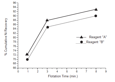
The practical flotation time required for an ore can be determined by producing incremental concentrates. Separate concentrates are removed at timed intervals (typically in geometric increments, e.g. 1, 2, 4, 8 minutes, etc. although any other time intervals are equally valid), until the froth is completely barren. Using the weights and assays for each incremental concentrate, the metal distribution in each can be determined. This information is then graphically plotted as cumulative recovery vs. cumulative flotation time to estimate the practical limit of flotation time. Different collector systems will often show significant differences in flotation rates, which will be apparent by comparing their individual recovery vs. time curves. It is also good practice to microscopically examine the incremental concentrates to determine the relative flotation rates of the variously associated minerals and the necessity for regrinding.
The rate at which the mineralized froth is removed and the position of the air valve will also have an influence on flotation kinetics. Therefore, it is advised that a fixed froth depth and a consistent froth scraping pattern at timed intervals, about every 15 seconds, be maintained. If a compressed gas cylinder (air or nitrogen) is to be used for flotation, an integral flow meter, to maintain a constant gas flow, may be installed between the gas source and the air inlet on the flotation machine. The impeller shaft and walls of the cell should also be periodically washed with process water from a wash bottle to return adhering minerals to the pulp and to maintain the pulp level.
For plant design purposes, it is usual practice to allow at least double the laboratory flotation time for the actual plant operation.
Technical Note. Fitting Flotation Kinetics Using Excel®.
The Machinery
In batch flotation tests, it is typical to assume Klimpel first-order flotation kinetics for the dependence of a given metal/mineral recovery on time (Mesa and Brito-Parada, 2019). Therefore, the cumulative recovery vs. cumulative time is given by the following:

Where R is the cumulative recovery after time t, R∞ is the maximum theoretical recovery, k is the first order time constant (in units of time-1) and t is the cumulative flotation time. More complex kinetics in which a “fast-floating” population of particles and a “slow-floating” population of particles can also be assumed as well as other more complex models, however, we will use the above-stated equation for illustration purposes.
From a set of flotation data in which concentrates were taken at 1, 2, 4 and 8 minutes, we are interested in fitting the kinetic equation and estimating both of the relevant parameters, namely, R∞ and k, for a given set of test conditions. Because the equation to be fitted is non-linear, in order to carry out a linear least squares minimization routine, one first needs to linearize the equation by expressing it as a Taylor expansion in the parameters as follows (truncated at the first order terms):

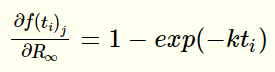
Where 𝒂i’s refer to the parameters in the equation; in our example we have two parameters, therefore, 𝒂0 = R∞ and 𝒂1 = k. The f(ti)j term refers to the estimated values and f(ti)j+1 are the predicted values. 𝚫𝒂o is the difference between an initial guess for R∞and a subsequently estimated value as will be shown below. The partial derivatives are evaluated at the corresponding estimated (and, later, updated-) parameter values, and for this particular example these partial derivatives are given by:
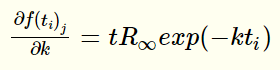
We subtract the estimated values, f(ti)j, from the measured yivalues to obtain:

Where ei’s refer to error terms. This last expression can be put in matrix terms as follows:

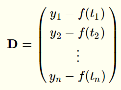
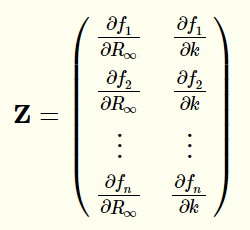
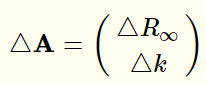
Note that n equals the number of experimental data points. The solution (i.e. the minimization of errors, ei) is carried out by solving the so-called normal equations of linear least squares regression to finally obtain:

𝜟A, the matrix on the left side of this last expression, is the one that allows us to update our estimates of R∞ and k, and by doing so iteratively, arrive at an optimum set of values. Although this last equation might seem a bit intimidating, it is straightforward to implement in Excel® as will be shown next.
The Application
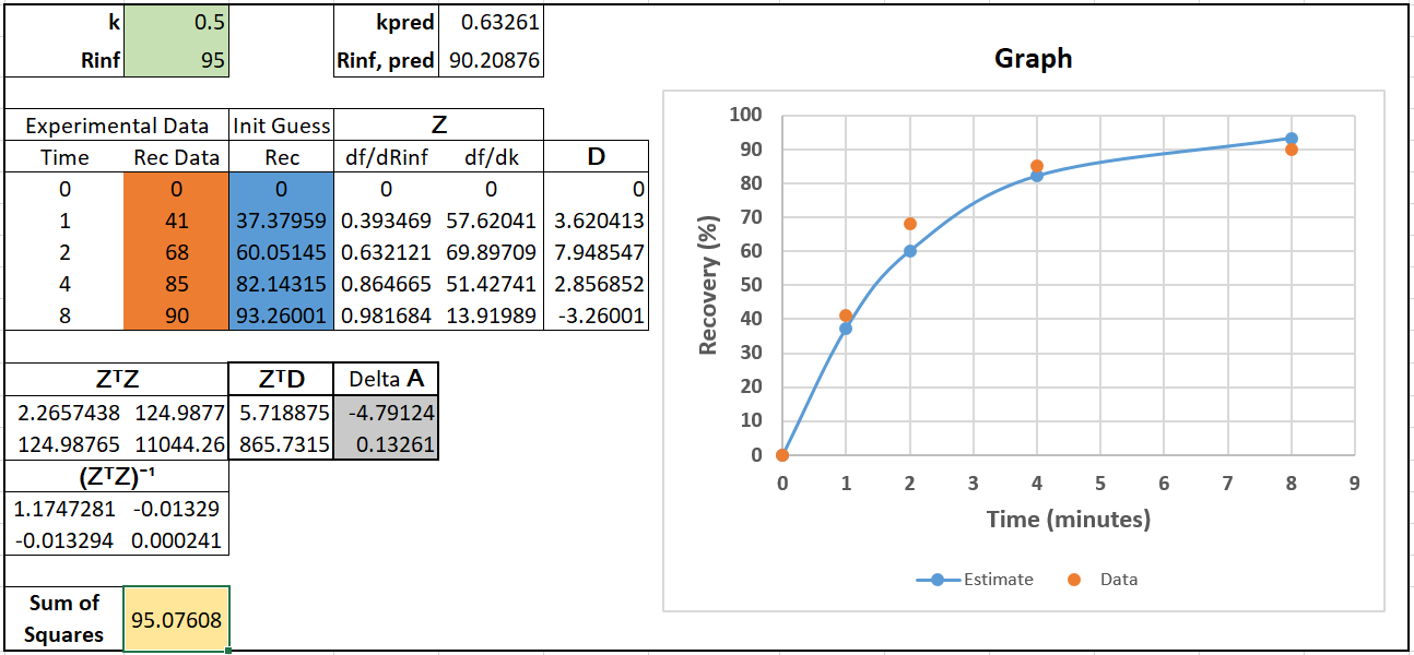
One first starts by populating the cells with the independent variable, i.e. time (t), as well as the experimentally-obtained recovery data (highlighted in orange in Figure TN1). One can then generate the fitting data by using the fitting equation with the corresponding time, as well as initial guesses for R∞ and k (these last two parameters are highlighted in green in the figure). The Z matrix is then built by entering the partial derivatives each in one column (again using the experimental time and the two initial parameter guesses). In addition, a difference matrix D is built whose entries are the difference between the experimental recovery values and the guessed fitting recovery values. A sum of squares field is also created with the values of D, such that D12 + D22 +...(cell highlighted in yellow). One can also create a graph with the experimental and fitted values to track the progress of the fitting routine as shown on the right of the figure.
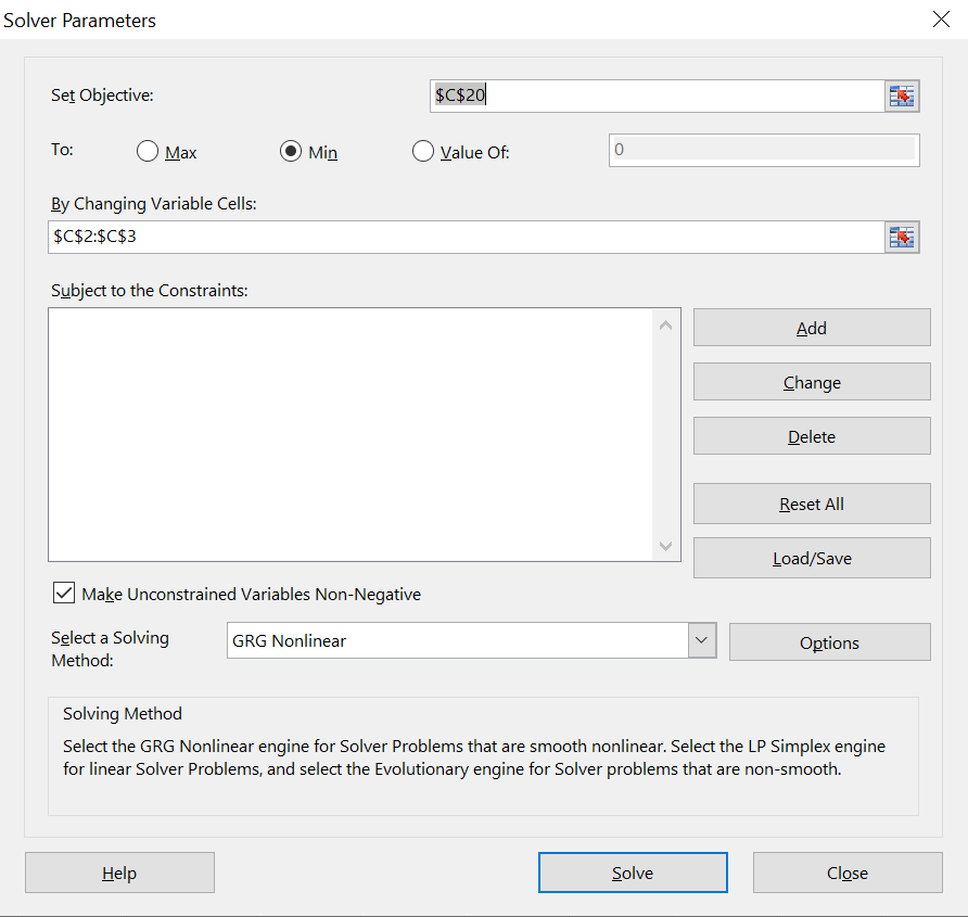
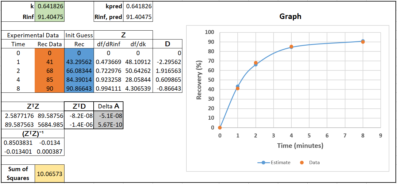
The next step is to carry out the matrix computations required to compute 𝜟A, namely, ZT, ZTD, ZTD, and [ZTZ]-1. The first three can be computed from the columns already generated and using Excel’s “SUMPRODUCT” function to do simultaneous element-by-element multiplication and summation. The inverse matrix ([ZTZ]-1) can then be computed by using Excel’s “MINVERSE” function on ZTZ. Next, [ZTZ]-1 is matrix-multiplied with ZTD to obtain 𝜟A (values highlighted in gray in the figure). The values of 𝜟A can be added to the corresponding initial parameter guesses. So, for example, for R∞,predicted = R∞, initial - 4.79124; for kpredicted = kinitial + 0.13261. These values are then entered into the green fields and the process is repeated until there is no change between predicted and initial values. However, we can automatically arrive at the best set of parameters values by using Excel’s “Solver” Add-In (Figure TN2), in which we minimize the “sum of squares” cell (cell $C$20 under “Set Objective” and choosing To: “Min”) by varying the two parameter cells (putting the green highlighted cells, $C$2:$C$3, into the “By Changing Variable Cells” field). The final answer should yield R∞,predicted = R∞, initial and kpredicted = kinitial as shown in Figure TN3.
Collectors
Establishing the optimum collector combination is generally regarded as one of the most important aspects of a metallurgical investigation. Although there are many individual collectors for sulfide minerals, the most widely used belong to the general chemical families such as dithiophosphinates, dithiophosphates, monothiophosphates, dithiocarbamates, thionocarbamates, thioureas, allyl xanthate esters, xanthogen formates, mercaptobenzothiozole and xanthates. Within each of these chemical families, there are many variations of alkyl or aryl groups which, particularly in the case of the dithiophosphates, can demonstrate significant differences in metallurgical performance on an ore. The metallurgist, therefore, should test at least a few variations within a particular chemical classification before making a judgment on its effectiveness. Syensqo has developed Select-A-Guide (an Expert System) to aid the metallurgist in choosing likely candidates for evaluation. One must also bear in mind that judgment of a collector's performance should not be made hastily, based on its lone use. Each of the chemistry/functionality associated with the collector molecule may have a selective affinity for a particular mineralogy. For example, combinations of different collector types, such as thionocarbamates with dithiophosphates, may demonstrate better metallurgical performance (synergism) than either collector used on its own. Complex ores contain various minerals and associations, therefore, one collector may not be adequate in providing the desired metallurgy.
Frothers
Selection of a suitable frother for plant operation, by means of laboratory testing, is more difficult than for other reagents to be used in the plant. Of particular interest is the ability of the frother to improve flotation kinetics, recovery and selectivity. The ideal frother or frother combination selected should produce frothing conditions, suitable for mineral transport to the froth phase and subsequent cell overflow, while also allowing drainage of entrained gangue particles. The type of flotation cell used in the plant; ore granulometry, the minerals present and their associations, and the presence of slimes will all have an influence on the frothing conditions and the froth character. It is usual practice to make the final frother choice by actual plant testing. For laboratory batch flotation tests, a froth depth of 1.5 to 3 cm is adequate.
Where selectivity in flotation is essential, the first choice of frother should be an alcohol type (i.e., AEROFROTH® 70, AEROFROTH® 76A, AEROFROTH® 88 or OREPREP® F-501 frother). Where stronger frothing conditions are required, use of a polypropylene glycol frother such as AEROFROTH® 65, or OREPREP® F-507 frother is recommended. In addition, Syensqo technical representatives can provide assistance in designing or recommending custom formulated frothers to provide optimum frothing conditions. For further information on the selection and use of frothers, please contact a Syensqo representative.
Modifiers
The presence of easily floating gangue minerals such as talc, chlorite, sericite, and pyrophyllite may require depressants such as AERO® 633 depressant, CYQUEST® 40E antiprecipitant, AERO® 8860GL GCA depressant, and various natural polysaccharides. Sodium silicate is sometimes used in sulfide mineral flotation as a dispersant. Carbonaceous matter can be depressed with AERO® 633 depressant. The polymeric depressants used in the selective depression and separation of various sulfide minerals are discussed under the headings for those ores and in Flotation Reagent Fundamentals .
Separate treatment of sands and slimes
In the case of ores with a high clay content (such as kaolin), dolomite, clinochlore or phlogopite, it may be advantageous to separate the ground pulp into a sand fraction and a slime fraction for separate flotation treatment.
For example, clay slimes increase pulp viscosity and interfere in the recovery of the coarser particles. The fine sulfides, minus ~20 µm, often float more slowly than the plus 10 µm particles, requiring a longer flotation circuit residence time.
In actual practice, there are two treatment schemes generally used. In the first method, the ground ore is separated into a sand fraction and a slime fraction for separate rougher flotation. In the second method, the ground ore is subjected to rougher flotation, followed by cycloning the rougher tails into sand and slime fractions. The sand and slime fractions are then treated separately by scavenger flotation. The coarse scavenger feed may require regrinding before flotation.
In addition the use of a dispersant such as sodium silicate, sodium hexametaphosphate CYQUEST® 3223 antiprecipitant, CYQUEST® 15 antiprecipitant and CYQUEST® 4000 processing aid will also help to disperse slimes and improve recovery.
Stages of flotation rougher, cleaner and scavenger
Laboratory flotation is a batch process that may consist of the following separation stages: rougher, scavenger and cleaner.
Rougher: the first stage of separation and concentration whereby recovery of the desired minerals is maximized while minimizing gangue flotation. The proper collector selection is critical in this regard.
Scavenger: tailings from rougher and, in some cases, recycled cleaner flotation tailings are floated, often with additional collector and frother, to maximize the recovery. The objective is to recover particles (i.e. middling) not recovered during rougher flotation.
Cleaner: the second stage of concentration, whereby the products of rougher and scavenger flotation are re-floated to maximize grade. In most cases, the rougher and scavenger concentrates are reground before cleaner flotation. Multiple cleaning (re-cleaning) stages may be necessary to obtain a marketable concentrate. Small amounts of collector are usually added to aid recovery.
One key aspect of flotation testing is the choice of cell size to use in a given test program. It needs to take into account the stages of flotation that will be carried out, the amount of ore available, the operational parameters (e.g. % solids), test objectives, etc.
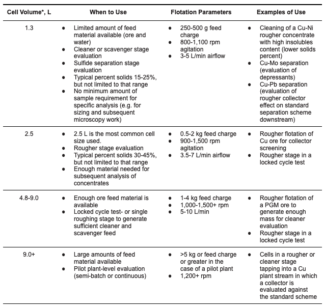
*Standard Metso cell volumes. Cell volume stated is that of liquid level 1” from the lip with Denver impeller/stator assembly in place.
Suppose for example, that a series of 25 collector screening rougher tests will be carried out and 15 kg of massive sulfide ore are available, a P80 grind size of 100 micron will be used, an average mass recovery of 15% is expected (as determined from diagnostic tests), the pulp solids content by weight will be 37% and the concentrate and tails will be sent for chemical analysis of Cu, Fe and S. One can then split the ore into 30 charges of 500 g, sample a charge to send for elemental analysis, and take another sample to measure the dry ore’s density, which turns out to be 3.1 g/cm3. Based on all this information, we determine that a 1.3 L cell is most appropriate; the solids % comes at about 37%.
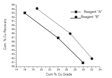
In most cases, simply conducting rougher flotation tests is not adequate to fully judge the performance of a collector, reagent scheme or the variable under study. Basing collector selection on rougher flotation recovery alone can be misleading. For example, a collector which gives the highest rougher recovery may be so unselective as to lead to high circulating loads and inferior recovery and concentrate grades in the cleaning stages. At the very least, rougher flotation collector evaluation should include a minimum of three concentrates taken over time to produce grade recovery curves, as shown in Figure 4. Selection of collectors for further testing should then be based on the relative positions of the grade-recovery curves.
It is good practice to carry rougher flotation into the cleaning stages to produce the final product and to completely evaluate the influence of the variable(s) on the total process. In order to have enough concentrate to conduct cleaner flotation, two or more rougher floats should be conducted. An alternative is to conduct rougher flotation using a larger pulp volume (2-3 kg of ore) and then to clean the concentrate in a smaller volume cell (0.5 to 1 kg). The downside to conducting batch rougher and cleaner tests is that the cleaner tails and process water are not recirculated, as they are in the plant and, thus, locked cycle flotation testing would more closely simulate plant practice.
Locked cycle flotation testing
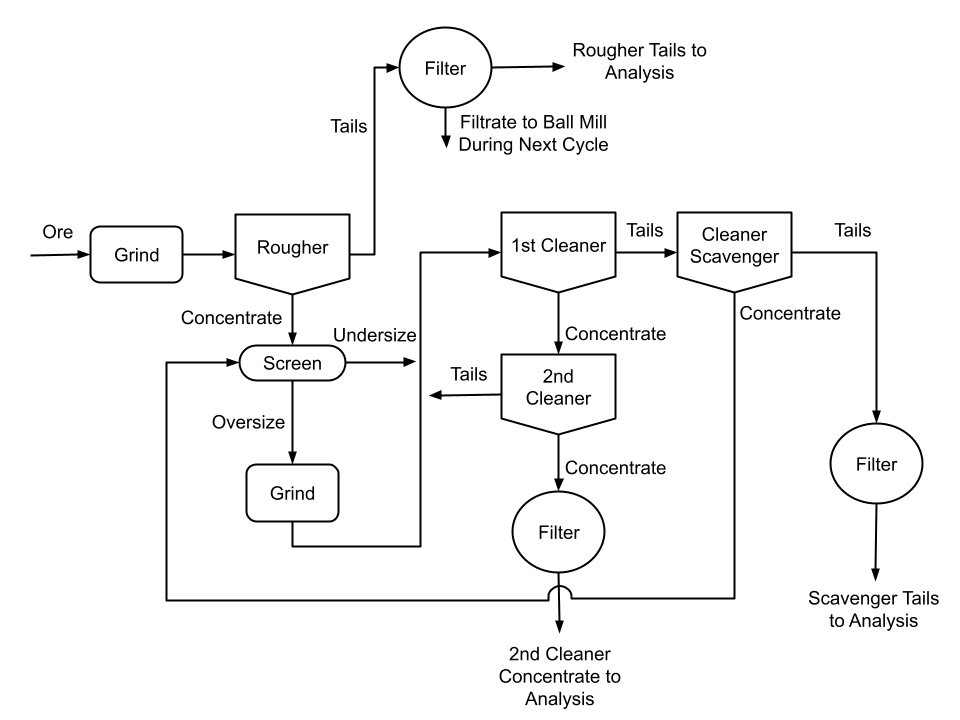
To complete the testing of an ore for flowsheet development and to obtain metallurgical data on expected plant performance, locked cycle flotation tests must be carried out. Prior to conducting such tests, the necessary conditions for regrinding of rougher or scavenger concentrates and intermediate products (cleaner tailings) should be established. The need for regrinding is determined by microscopic inspection of the various flotation products, as described previously.
In each complete cycle test (Fig. 5), middlings (in the form of cleaner tailings or scavenger concentrates) are recirculated back one or more processing steps in the subsequent test cycle. The disposition of these middlings streams should be determined during prior laboratory flotation tests and by optimization during the locked cycle test work. The results of the locked cycle tests may indicate that a change in the middlings flow may be required.
From each cycle test, a final concentrate and final tailings are obtained. Except for the very last cycle test, middlings will be re-circulated. An estimate of middlings weights can be made by filtering the middlings products and obtaining their weights as damp filter cakes. In this manner it can be determined if middlings weights stabilize after a few complete cycles. It may take from four to seven cycles to reach equilibrium conditions.
Equilibrium is reached when, for at least two consecutive cycles:
- The combined weights of the final concentrate plus the final tailings stabilize and approximate the weight of fresh ore charged to each new cycle.
- The assays of the final concentrate and the final tailings stabilize and the calculated head assay, based on these two products, is similar to the original fresh feed assay.
- Metallurgical distribution between the final concentrate and the final tailings stabilizes.
If equilibrium conditions are not established after six or seven cycles, the flotation products must again be examined microscopically to determine the cause. Addition of a small amount of collector to the cleaners, or further regrinding of middlings products may be required. The use of recycled process water can be simulated by clarifying the tailings by sedimentation to recover the water. Water from the concentrate or intermediate products can be recovered in the same way, or by filtration. The effect of reagents and soluble salts in a recirculating water system can also be assessed in this manner.
Where more than one valuable metal is to be recovered, each into a separate concentrate, the complexity of the cycle test and calculations increase considerably.
Handling of Flotation Products
Flotation products are filtered using vacuum filtration for the concentrates and a large volume pressure filter for the tailings. We suggest using filter paper of high wet strength such as sharkskin filter paper or craft paper. Filtration can further be enhanced by flocculating the products, which is extremely beneficial if the products contain a large amount of clay or slimes.
The filtered products are then oven dried at 70-100°C. It is important that the oven temperature does not exceed 100°C, so as to avoid roasting the sulfide minerals and driving off sulfur. The concentrate and tails should be dried separately, either in separate ovens or if in the same oven, by placing the low grade tails on the upper shelves and the higher grade concentrates on the lower shelves.
After drying, the net weight of the flotation products is recorded for calculating the metallurgical balance. The products may be brushed through a screen (35 Tyler mesh for example) to break up aggregates, and then mixed by rolling on a rubber sheet, before representative cuts are taken for chemical analysis.
The cuts should be placed in a sealable plastic bag or envelope and labeled with the relevant test information (test number, sample type, etc.). Samples sent to an assay lab are usually pulverized prior to analysis, therefore, any samples needed for microscopy work should be taken before assays are conducted. This is to maintain the integrity of the minerals and their associations.
Assaying and Interpretation of Results
Assaying
The incremental concentrates and the tail sample from flotation must be filtered, dried and weights recorded, and then submitted for assay. Appropriate analysis of the flotation products is of paramount importance. Poor handling of the flotation products, resulting in cross contamination, can lead to erroneous results and conclusions. Selection of a highly qualified assaying facility, with experience in analyzing various powdered samples for the desired elements (Cu, Au, Mo, Pb, etc.), will reduce re-work or prevent nullification of whole test programs all together.
Interpretation of results
The assay results and recorded weights are then used to generate mass balances from which graphs can be created.
- Rate kinetic curves can be generated, time versus % cumulative recovery (see Figure 6).
- Grade recovery curves, % cumulative grade versus % cumulative recovery (see Figure 4).
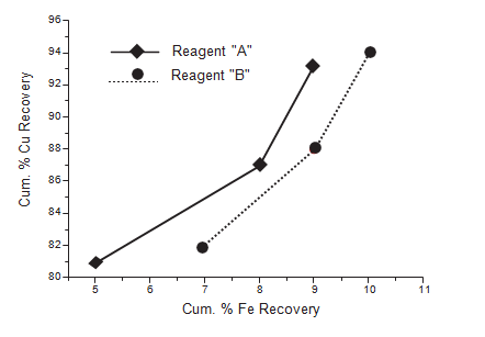
- Selectivity curves, % cumulative recovery gangue/penalty metal versus % cumulative recovery valuable metal (see Figure 7).
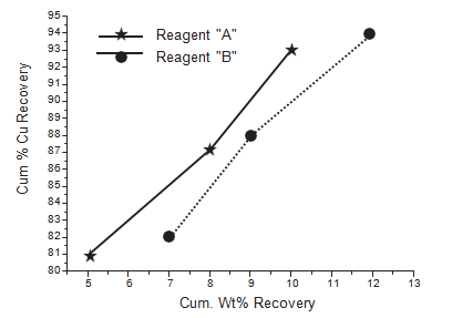
- % Mass Recovery versus % Recovery (see Figure 8).
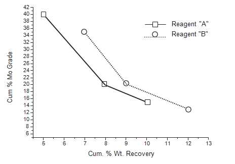
- % Mass Recovery versus % Grade (see Figure 9).
The Effects of Reagent Choice on Flotation Circuit Design and Operation
When testing a new ore body, the potential impact of reagent choice on equipment selection and circuit configurations is often not fully appreciated. During preliminary feasibility testing, it is not uncommon to evaluate only one or two collectors (usually a xanthate and/or a dithiophosphate), an arbitrarily selected frother, and a pH modifier such as lime. This is particularly true in the case of relatively simple ores such as a copper or copper-gold ore containing iron sulfides such as pyrite. The assumption is that this will provide sufficient information for flowsheet design and a preliminary economic/metallurgical analysis. "Fine tuning" of reagents is left to a later stage of the investigation, or even until after the plant has started operating. We believe that, even for simple ores, this approach has potentially serious pitfalls, which are discussed in this section. Different reagents (including collectors, frothers, pH modifiers, and depressants) can have a significant effect on flotation kinetics, the grade-recovery relationship, the amount and type of froth, the mass of rougher and scavenger concentrates, and rejection of penalty elements, etc. Optimization of these variables at an early stage of the testing process can have a significant effect on flowsheet design, as well as on capital and operating cost estimates. Consider a situation where Reagent combination "A" gives the highest rougher-scavenger recovery, but with a lower concentrate grade (and hence a greater mass of rougher-scavenger concentrate) than Reagent combination "B". If combination "B" is then eliminated from further consideration because it gives lower rougher recovery, its following potential benefits of better rougher selectivity may be overlooked:
- The greater selectivity of Reagent "B" and the lower mass pull in the rougher-scavenger circuit will reduce the required regrinding and cleaning capacity, which may reduce both capital and operating costs.
- The reduced load in the regrind and cleaning circuit may well result in an increase in final concentrate grade and/or recovery compared to Reagent "A".
- Reduced circulating loads in the cleaner circuit usually mean the cleaner circuit is easier to control and operate.
- The use of a more selective reagent or reagent combination in the rougher-scavenger circuit usually enables operation of that circuit at a lower pH, thus reducing the amount of lime or other depressant required.
- The use of a selective collector may produce a sufficiently high-grade concentrate in the early stages of the rougher circuit, that this product can bypass the regrinding stage and be sent directly to the feed to the first or second cleaner. This not only further reduces the load on the regrind circuit, but also minimizes the risk of over grinding already liberated value minerals. Such over grinding can lead to "sliming" and subsequent loss of overall recovery. Flowsheets 1 and 2 are traditional, simple flotation circuits. Flowsheet 3 indicates the kind of circuit which may be possible when using more selective reagents.
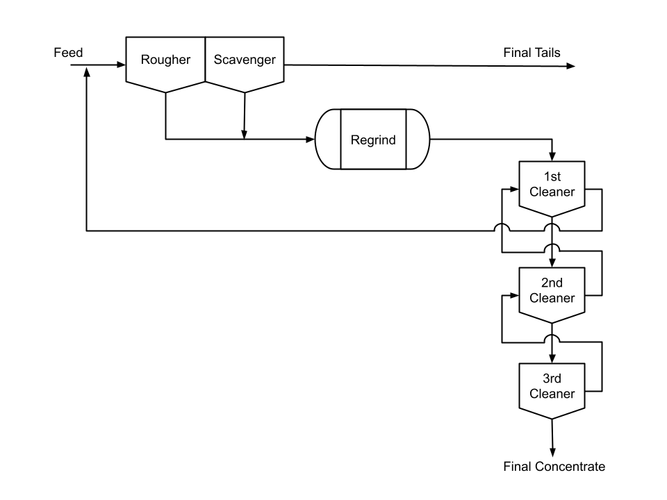
Flowsheet 1 is typical of early base-metal flotation flowsheets. The cleaning circuit is totally "closed" with the 1st cleaner tails being returned to the head of rougher-scavenger flotation. In some cases, the scavenger concentrate was also returned to the head of rougher flotation. Such a flowsheet is typified by high circulating loads in both the rougher-scavenger and cleaner stages.
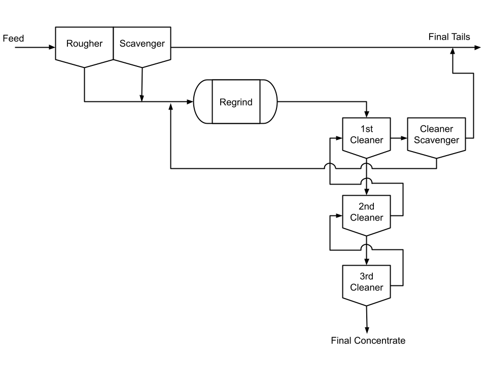
Flowsheet 2 is probably the most typical of current base-metal flotation circuits. The 1st cleaner tailing is sent to a cleaner-scavenger stage, the concentrate of which is returned to the regrind mill. The cleaner-scavenger tailing joins the rougher-scavenger tailing to form the final plant tailings. This design reduces the circulating loads in both the rougher-scavenger and cleaner stages, thereby reducing the flotation capacity required for a given mill tonnage.
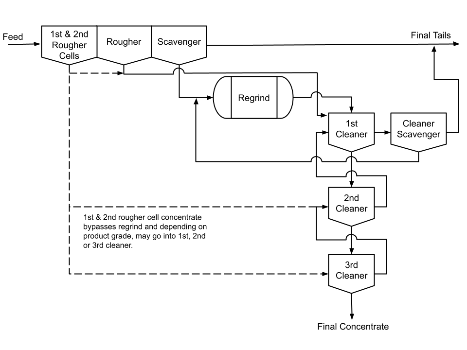
Flowsheet 3 represents the type of design which may be made possible by the use of more selective collectors in the rougher-scavenger stage. Samples of the concentrate are taken from successive cells down the rougher bank for both chemical assay and mineralogical examination. In most cases, it will be found that the concentrate from the early stages of rougher flotation will be of high enough grade and sufficiently liberated to bypass the regrind mill. Whether this concentrate is sent to the first, second, or final cleaner stage will depend upon its grade and mineralogical characteristics. This flowsheet design further reduces the circulating load in the cleaners as well as minimizing over grinding of already liberated value mineral. The advantages described above for simple ores are even more important when treating complex ores containing two or more value minerals. With these ores, separation efficiency between the individual value minerals is often more critical than the selectivity between the value minerals and the gangue minerals.
In the case of already existing flotation circuits, many of the described advantages could still be obtained if suitable circuit and piping changes were made. Furthermore, since many plants are already operating at or above design tonnages, greater selectivity in the rougher circuit and the consequent reduction of the load on the regrind and cleaning circuit can have major benefits, such as eliminating circuit bottlenecks.
To summarize, the selection of collector and other reagents should not be based on rougher-scavenger evaluation only, and certainly not solely on reagents that give the highest recovery therein. Rather, reagents should be evaluated on the grade-recovery relationships they produce throughout the whole process, including regrinding and cleaning. This will inevitably entail at least locked-cycle testing in the laboratory, preferably followed by pilot-scale testing and plant testing.
Bibliography and References
- Crozier, R. D., 1992. Flotation, Theory, Reagents and Testing. Oxford: Pergamon Press.
- Booth, R. B., 1954. "Flotation". Ind. Eng. Chem. (1954), 46, 105-11.
- Fuerstenau, D.W. ed. 1962. "Froth Flotation" – 50th anniversary volume, New York: AIME.
- Gaudin, A. M., 1939. Principles of Mineral Dressing. New York: McGraw-Hill.
- Glembotskii, V.A., V. I. Klassen and I. N. Plaksin, 1963. Flotation. New York: Primary Sources.
- Hartman, H. L., 1992. SME Mining Engineering Handbook. 2nd ed. 2 vols. Littleton: SME.
- Mesa, D., Brito-Parada, P.R. Scale-up in froth flotation: A state-of-the-art review. Separation and Purification Technology, Volume 210, 2019, Pages 950-962. https://doi.org/10.1016/j.seppur.2018.08.076.
- Mular, A. L. and R. B. Bhappu. 1980. "Mineral Processing Plant Design". 2nd ed. New York: AIME. Chapters 2 and 3.
- Nagaraj, D.R. and A. Gorken, 1991. "Potential controlled flotation and depression of copper sulfides and oxides using hydrosulfide in non-xanthate systems". Canadian Metallurgical Quarterly vol. 30, No. 2, pp. 79-86.
- Nagaraj, D. R. and F. Bruey, 2002. "Reagent Optimization: Pitfalls of Standard Practice". Workshop/Conference on Flotation and Flocculation, Hawaii, USA.
- Perry, J. H., 1963 Chemical Engineers Handbook. New York: McGraw-Hill.
- Sutherland, K. L. and I.W. Wark. 1955. "Principles of flotation". Melbourne: AIMM.
- Taggart, A. F., 1945, Handbook of Mineral Dressing. New York: McGraw-Hill.
- Trahar, W. J., 1981. "A rational interpretation of the role of particle size in flotation". Int. J. Min. Proc., 8, 289.
- Weiss, N. L., 1985, SME Mineral Processing Handbook. 2 Vols. New York: AIME. Vol. 2, Section 30.
- Wills, B. A., ed. 1997. Mineral Processing Technology. 6th ed. Oxford: Butterworth-Heinemann.