
Introduction
Flotation, though simple in concept as a separation/concentration unit operation is, at a fundamental level, a rather complex process. In fact, flotation is an interplay between multiple physicochemical and purely physical sub-processes. These subprocesses span a wide range of sizes, from the angstrom to nanometer scales of molecular phenomena, up to the micron to centimeter range of ore particles and bubbles, to even the meter sizes of flotation equipment, all of which work together to result in an effective separation between value and gangue minerals. This fact alone clearly indicates that both physical and chemical factors are equally important in flotation. In other words, it would be naïve to proclaim that one set of factors is more important than the other set, which is sometimes done in research or practice. Chemical factors include the interfacial chemistry involved in the three phases that exist in a flotation system solid, liquid and gas. Interfacial chemistry, in turn, is dictated by all of the flotation reagents – such as collectors, depressants, frothers, activators, and modifiers – used in the process, water chemistry, and the chemistry of the minerals. Physical (or more accurately, physico-mechanical and operational) factors comprise equipment components (cell design, hydrodynamics, bank configuration, and bank control) and operational components (feed rate, mineralogy, particle size, air flow rates, cell pulp levels, and pulp density). Thus, flotation is a complex process in practice, involving many scientific and engineering phenomena.
In most flotation systems, physical and chemical factors are not independent, i.e., there are significant interactions among the many variables. In theory, when all physical factors are optimized, a change in a chemical factor should clearly record a measurable change in flotation efficiency (either recovery or grade or both), and vice versa. In practice, however, this may not be immediately obvious because of certain operational restrictions, and metallurgists have to revert to statistical tools to demonstrate significant changes. A further complication is that neither physical nor chemical factors can always be fully or satisfactorily optimized, since there can be significant changes occurring routinely in mineralogy, feed rates and particle size distribution. Nevertheless, flotation plant operators still achieve impressive separations and performance by managing controllable factors.
In general, in a fully commissioned plant, it is more difficult to change physico-mechanical factors than chemical or operational factors. Indeed, in most plants considerable attention is, therefore, focused on changing or optimizing chemical and operational variables.
Chemical Factors
The importance of chemical factors in achieving target performance has been widely recognized. In many circuits, a mere change in pH of the pulp can cause dramatic differences in flotation efficiency. This is true of flotation reagents, as well.
In this section, an attempt is made to highlight how changes in the chemistry of flotation reagents can have marked influence on flotation efficiency. The chemistry of collectors is used to illustrate structure-performance aspects, though the principles are applicable to depressants as well.
A brief, simplified description of terminology will be necessary to appreciate the structure-activity aspects of flotation reagents. Donor atoms, donors or ligand atoms are those atoms in the reagent molecule that bond directly with the metal atom on the mineral surface. Ligands are the functional groups containing the donor atom(s) on the reagent molecule that participate in bond formation with metal atoms on the mineral; donor atoms are also often referred to as ligands. Functional groups are a well-recognized group of atoms containing the donor atoms in the reagent molecule. Acceptors are atoms or groups of atoms that accept electrons from donors. A metal atom on the mineral surface is the acceptor in most instances. Acceptors are generally positively charged, while donors or ligands or functional groups are often negatively charged. Note, however, that in cationic flotation reagents, the functional group of the molecule carries a positive charge, and this can interact with a mineral surface that has negative sites. Functional groups are generally polar (i.e., carrying a charge, partially or fully). Non-polar moieties of a flotation reagent molecule are generally a hydrocarbon chain (linear or branched, aliphatic or aromatic or a combination).
For a vast number of flotation reagents, adsorption at the solid-liquid interface is of critical importance. Frothers, which adsorb significantly at the liquid-air interface and alter its properties, can also adsorb at the solid-liquid interface and influence flotation outcome. However, interfacial chemistry of frothers is largely characterized by non-specific adsorption processes. Most commonly used frothers belong to the classes of short-chain alcohols and polyglycols (and their monoethers). Consequently, the scope of structure-activity relationships is rather limited relative to collectors, however, activity can be tuned by varying the level of branching in the alkyl/non-polar portions of molecules, the position of hydroxyl groups, number of ethylene (or propylene) glycol units, etc.
The driving force for, and the mechanism of, adsorption of flotation reagents on minerals comprises chemical (chemisorption, surface reaction or complexation, and chemical adsorption), electrostatic (physisorption or physical adsorption), and non-specific forces (such as Van der Waal's forces, hydrogen bonding, and the so-called hydrophobic force). Chemical interactions have the highest adsorption energies, followed by electrostatic and non-specific interactions. In many cases, more than one driving force is in operation. Overall adsorption energy is, therefore, a sum of all energies associated with various adsorption processes.
In the case of non-specific adsorption processes, structural aspects of the reagent molecule that can be changed include the nature and type of the hydrocarbon chain, moieties capable of hydrogen bonding, etc. In general, such changes in the molecule can only cause small changes in interfacial properties (for example, hydrophobicity) of the solid-liquid interface. Hydrophobicity imparted by a reagent on the mineral surface increases with an increase in the reagent's hydrocarbon chain length.
When the adsorption process is predominantly electrostatic in nature, a change in the charge density of the molecule (or the functional group), or of the mineral surface, causes a noticeable change in adsorption energy or interaction energy. Pulp chemistry plays a significant role in these systems; for example, the presence or addition of inorganic ions. Reagents that carry positively charged functional groups are called "cationic" reagents; these are typically amines – primary, secondary, tertiary or quaternary. Reagents that carry negatively charged functional groups are called "anionic" reagents; examples of these are fatty acids (carboxyl groups), hydroxamates and alkyl or aryl sulfonates (or sulfates). Reagent molecules that can potentially have both cationic or anionic sites (depending upon pH, for example) are called "amphoteric" (zwitter ionic) reagents. In general, for cationic reagents, adsorption is predominantly electrostatic. Similarly, in the case of sulfonate or sulfate-containing reagents, the electrostatic component is usually the predominant one (there can, however, be a chemical component also). In the case of anionic collectors containing carboxyl or hydroxyl groups, there is often a significant chemical component in the overall adsorption energy, in addition to the electrostatic component. Under certain conditions, for these reagents the electrostatic component can be completely overridden by the chemical component.
Structure-activity aspects become very important, and offer a wide scope for reagent design and control in systems where the driving force for adsorption of flotation reagents on minerals is chemical. Since chemical interactions between reagent molecule and mineral surfaces have the highest adsorption energies, changes in structure of the reagent molecule can potentially result in large changes in the strength of adsorption, the resultant interfacial properties, and flotation response. This has been clearly demonstrated in a large number of reagent families in flotation research and practice. A few examples are given later in this section.
Several models have been proposed to explain chemical adsorption of reagent molecules on mineral surfaces. Some examples of these include chemisorption, surface reaction, and surface complexation. Irrespective of the model or the process of chemical interaction of reagents with minerals, the basic requirement is that a chemical bond – covalent or partially covalent – be formed between the donor atoms of the reagent and the metal atom of the mineral, at least in the first adsorbed layer. Further, in the first adsorbed layer, the metal atom is still a part of the mineral lattice. Subsequent layers of metal-reagent complexes can, and often do, exist, but in these layers the metal is obviously not part of the mineral lattice6. The first adsorbed layer is quite stable on the mineral surface, and often requires chemical changes for desorption; the common notion that high turbulence can dislodge adsorbed species is a myth, given that, at molecular scales, inertial forces are not relevant relative to thermal and chemical forces and, therefore, the latter dictate a molecule’s behavior. In the case of sulfide minerals and certain thiol reagents, an electrochemical mechanism of adsorption via formation of a metal reagent complex is now widely accepted13. Many sulfide minerals are excellent conductors and exhibit properties that are similar to those of metals. Electrochemical reactions are quite facilitated, and are similar to reactions in batteries or corrosion processes. Furthermore, many thiol reagents exhibit redox reactions. Extensive studies and plant observations have established that redox conditions of flotation pulps do influence flotation efficiency.
In discussing the chemistry of flotation reagents, it is most convenient to classify them into two distinct groups: a) those used specifically for sulfide minerals, and b) those used for non-sulfide minerals. With the exception of a few elements such as the base and precious metals, most elements or their minerals are obtained from non-sulfide ores. It is well recognized that separation schemes for non-sulfide minerals are distinctly different from those for base metal sulfide minerals.
Such distinctions can be readily understood by the fundamental differences that exist in physical and chemical properties between sulfide and non-sulfide minerals. These differences arise, for the most part, from differences in the chemistry between S and O. The base-metal sulfide minerals are characterized by mostly covalent or metallic bonding, low solubility in water, weakly hydrated surfaces and poor hydrogen bonding, a high degree of natural hydrophobicity, strong affinity for S-containing ligands, and pulp chemistry dominated by electrochemical reactions. Conversely, the non-sulfide minerals are generally characterized by ionic bonding, higher solubility in water, strongly hydrated surfaces and strong hydrogen bonding, strong affinity for O-containing ligands, and pulp chemistry dominated by ion exchange reactions. Plant practice is often consistent with the major differences between sulfides and non-sulfide minerals. Table 1 summarizes these major differences for the two mineral types.
| Property | Sulfarghides | Non-sulfides |
| Bonding | Mostly covalent (e.g. S-S, C-O, S-O) | Mostly ionic (e.g. Mg-O, Ca-O, Na-O) |
| Stoichiometry | Low | High |
| Solubility | Low | High |
| Stability | Oxidation | Hydration |
| Hydrogen bonding | Low | High |
| Surface property | Metal-like characteristics of S | High charge; strong acid-base characteristics of O |
| Affinity for donors in flotation reagents | Strong affinity to S-containing ligands | Strong affinity to O- and N-containing ligands |
The sulfur atom on either a carbon or a phosphorous atom in a molecule is the key donor and the center of activity in sulfide collector chemistry. Its bonding properties are readily modified by neighboring atoms and groups, especially by the two other major donor atoms N and O. Sulfide minerals can be floated by almost any collector, including those that do not contain sulfur. However, in order to obtain selectivity that is meaningful in industrial flotation at economic levels, a sulfur-containing collector is invariably preferred. This statement is amply supported by the fact that all of the commercially used sulfide collectors, since the introduction of xanthate, contain sulfur.
In addition to the basic functional groups containing the major donor atoms, substituents attached to them provide a unique character to the collector molecule. These groups essentially modify the affinity of the collector for a given sulfide surface, the hydrophobicity conferred, kinetics of adsorption, and the pKa of the molecule which, in turn, has a direct influence on the solution properties of the collector and its interaction with sulfide surface. Substituents can also participate in bond formation with the mineral, which may either reinforce or counter the interactions of the basic functional group with the sulfide surface.
Thus, seemingly minor changes to the structure of a collector molecule can have a very significant effect on the collector's performance in the flotation process. This is illustrated in the examples which follow.
Example 1. Functional group modification: change of chelation properties.
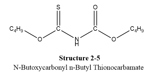
In the case of the traditionally used dialkyl thionocarbamates, such as O-isopropyl N-ethyl thionocarbamate (IPETC, AERO® 3894 promoter, Structure 2-1), the basic functional group is -O-C(=S)-NH-. An interesting modification of the basic dialkyl thionocarbamates is the substitution of an alkoxycarbonyl group on the N atom (as shown in Structure 2-2). The use of the strongly electron-withdrawing alkoxycarbonyl substituent introduces an additional active donor, O, in the form of C=O attached to the alkoxy group. Thus, the functional group is not solely restricted to the thionocarbamate; instead, it is the more complex -O-C(=S)-NH-C(=O)-O, which has quite different properties from the basic thionocarbamate group. The pKa of the molecule is directly affected; for example, the pKa of IBECTC (Structure 2-
2) is 10.5 compared with a pKa of >12 for IPETC. These attributes make the new thionocarbamates strong copper sulfide collectors at low pH values (<11), for example, while still maintaining the selectivity against pyrite characteristic of the thionocarbamates.
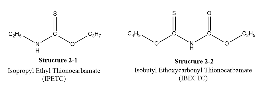
Fundamental studies have shown that the new alkoxycarbonyl thionocarbamates form a highly favored, six-membered chelate (see Structure 2-3) with Cu atoms on a copper sulfide mineral surface. In the case of IPETC, however, such a favorable chelate is not possible. Instead a less favorable four-membered chelate involving the O and the S is formed (see Structure 2-4). External reflectance FTIR studies using copper foils have indicated that when a copper foil was first treated with IBECTC and then with IPETC, the IBECTC adsorbed on copper foil could not be displaced by IPETC. When the copper foil was treated in the reverse order, IBECTC was able to adsorb on copper by displacing IPETC. Similar results were obtained when a xanthate was used instead of IPETC.
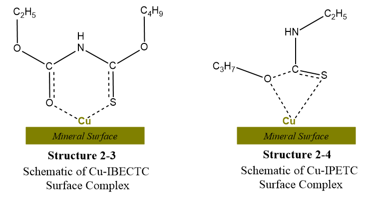
Recent studies by Syensqo have shown that chemical structures such as IBECTC although exhibiting superior metallurgical performance may be prone to environmental and safety concerns. However, our studies have shown that eliminating the branching in the structures and making both alkyl groups the same, these compounds not only become environmentally and safety friendly but also improve their metallurgical performance. One example of such structures is N-butoxycarbonyl-n butyl thionocarbamate (Syensqo's AERO® XD5002); illustrated in Structure 2-5.
Example 2. Functional group modification: addition of allyl pendant group.
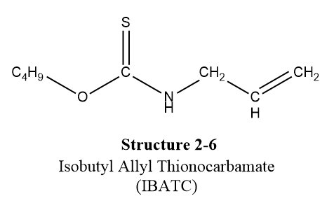
Another interesting modification of the dialkyl thionocarbamate structure is obtained by incorporating an allyl group, -CH2-CH=CH2 on the N donor atom (see Structure 2-6). The allylic double bond modifies the adsorption and collector properties quite significantly, in comparison to the dialkyl thionocarbamates such as IPETC. The double bond in allyl thionocarbamates can be expected to form a complex with Pt, Pd, and possibly Cu. Adsorption studies have shown that there is a strong tendency for the allyl thionocarbamates to interact with copper and platinum surfaces. Syensqo introduced the allyl thionocarbamates in 1980, and they were fully commercialized in 1989 (AERO® 5000 promoter series). One of their main attributes is the rapid flotation kinetics that they provide at quite low dosages. Laboratory and plant tests conducted on platinum ores have shown that the allyl thionocarbamates improve recovery of PGMs, again at low dosage levels.
Example 3. Functional group modification: change in donor atom.
 |  |
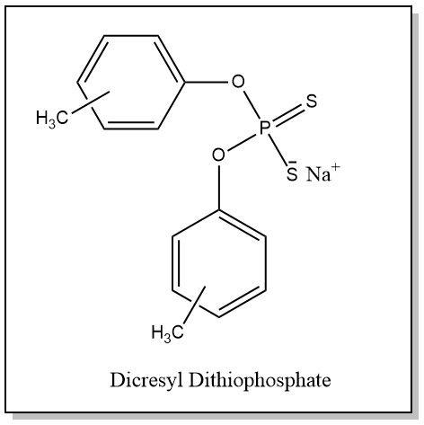 | 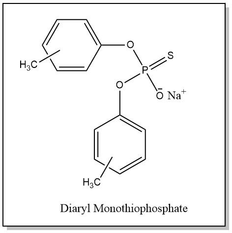 |
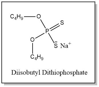
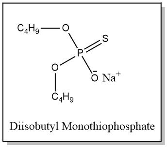
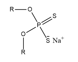
An important modification of the basic dithiophosphorous group, >P(=S)S, as found in the dithiophosphate collectors (Structures 2-7 and 2-9), is that of replacing one of the S donors in the functional group by an O donor to give the corresponding monothio derivative (Structures 2-8 and 2-10). This single change in the nature of the donor atoms in the dithioacid is sufficient to alter its collector property dramatically in view of the quite different properties of the donor atoms O and S.
Extensive studies of the solution and collector properties of the monothio and dithio acids in a wide pH range have indicated that the monothioacids are more stable, stronger acids, and stronger collectors than their dithio analogs under certain pH conditions. The dialkyl monothiophosphate, for example, is found to be a truly acid circuit collector (effective in the pH range 2-7 in contrast to the dithiophosphate, which is a better collector in the alkaline pH range (pH > 9).
The differences in the collector properties between the mono and dithiophosphates are attributed to the rather interesting tautomerism that exists in monothiophosphate (Structures 2-11 and 2-12). The available evidence suggests that, in aqueous solutions, the thiol form, P(O)SH, may be stable in the acid pH range and the thione form, P(S)O-, stable under alkaline conditions. The thiol form is understandably favorable for sulfide flotation.
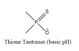 | 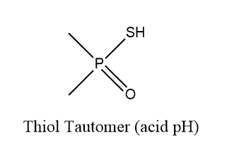 |
In the thione form, the very electronegative O tends to retain much of the electron density at the expense of the less electronegative sulfur. The reduced electron density on the thione S is probably responsible for weak bonding with sulfides above pH 7.
Monothiophosphates, introduced in 1989, are now used widely on copper and gold ores. The monothiophosphates are used for bulk sulfide flotation in acid circuits where they are more stable and stronger than xanthates, dithiophosphates, and xanthogen formates. They have also found application for selective gold flotation from primary Au ores or for improving Au recovery in base metal sulfide flotation in alkaline circuits.
Example 4. Pendant group modification: aryl vs. alkyl.
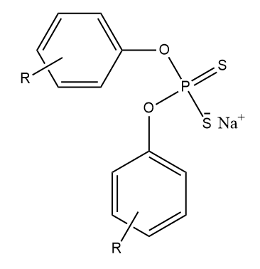
Often, enhanced performance can be realized by merely changing the hydrocarbon part of the reagent molecule, while keeping the functional group intact. For example, a slightly branched hydrocarbon group in a collector molecule can provide a greater selectivity in flotation than a linear hydrocarbon group, presumably due to the added steric hindrance imparted by the branching of the hydrocarbon group potentially reducing the molecule’s extent of adsorption on less favored mineral surfaces. Another example is that of a change in affinity for a given mineral when substituting alkyl to aryl hydrocarbon groups. For example, it is well known in flotation practice that an aryl dithiophosphate floats galena far better than an alkyl dithiophosphate (see Figure below).
 |  |
Example 5. Functional group modification: modulating selectivity.
It is well-known that fatty acids (Structure 2-17), which are used extensively in flotation of non-sulfide minerals, are inherently non-selective. Hydroxamic acids (Structure 2-15), which are structurally similar to fatty acids, are considerably more selective. They differ from fatty acids by a nitrogen, which does not participate directly in bonding with a metal atom, but has an effect on the electron density on the O donor attached to it.
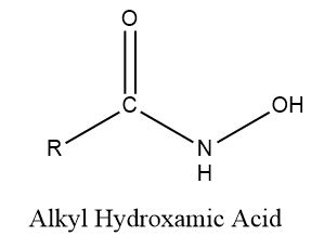 | 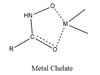 | 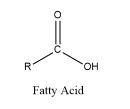 | 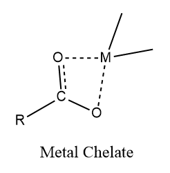 |
The O donors in hydroxamic acids are weaker donors (more selective) than those in fatty acids. There is considerable covalence in the bonds formed with metals (compared with the ionic character of the bonds formed with fatty acids). These factors impart considerable selectivity in the hydroxamate interaction with metals, and hence in flotation. They form five-membered metal chelates (shown in Structure 2-16) because the hydroxyl attached to N is appreciably acidic; this is in contrast to the fatty acids which, under certain conditions, can form a less stable four-membered chelate (structure 2-18). On the basis of differences in stability constants of many hydroxamic acid metal complexes, it can be predicted that hydroxamic acids should be more selective than commonly used fatty acids, and indeed this has been found to be the case in practice. A new manufacturing process was developed and alkyl hydroxamate was introduced by Syensqo in 1989 under the trade name AERO® 6493 promoter, which is currently used for the removal of colored impurities from kaolin and for oxide copper recovery. There is also a new series of improved alkyl hydroxamates commercialized under the name AERO® OX-100 with great performance and less impact on the froth. It was also shown recently that alkyl hydroxamates improve the recovery of precious metals that are associated with pyrite, marcasite, pyrrhotite and goethite. In kaolin beneficiation, alkyl hydroxamates have been found to be much more effective than fatty acids; they produce higher brightness clays with better yields from a variety of kaolin clays. No activators are required, and retention times in flotation are shorter than those for fatty acids.
Altogether, the design and use of collectors (or depressants) aims at selectively increasing the hydrophobicity (or hydrophilicity) of minerals of interest through adsorption of the reagents at the solid-liquid interface; this is a clear example of molecular scale agents, representing a chemical factor, whose action results in physical changes at larger scales. Clearly, adsorption is only one of multiple molecular, meso- and macroscale subprocesses that together result in successful mineral separations through flotation. However, practically and at the plant level, one can only hope to assess the efficiency of these subprocesses indirectly (and consequently in a phenomenological manner) through a few macroscale parameters characteristic of the ore feed reaching the flotation cell, the pulp zone hydrodynamics and the froth phase. The following gives details on these physical factors and how they are measured.
Physical Factors (Operational Variables)
Flotation is a complex process that is not only controlled by physicochemical parameters or variables discussed in the previous section, but also by operational aspects associated with the fluid dynamics of the flotation circuit. These include probabilistic aspects of particle bubble interactions, the kinetics of collector absorption and mineral particles removal through the froth phase. Therefore, one can characterize the efficiency of the flotation processes within both the pulp and froth phases through various means. The following details some of the approaches taken practically at the plant level.
Fundamentals of floatability
Floatability can be defined as the 'amenability of attachment between mineral particles and air bubbles'. It is not a flotation rate constant, however it can be used to estimate the rate of the flotation process by using the following equation:
$k = P \times S_b \times R_f$
where k is the first order flotation rate constant (in units of s-1), P is the ore feed floatability (a dimensionless number), Sb is the bubble surface area flux (in units of s-1) and Rf is the froth recovery (dimensionless fraction). The above expression for k can be conceptualized by thinking that the rate constant depends directly on a property of the incoming stream (P) together with those of the pulp zone (Sb) and the froth zone (Rf), respectively11. One, therefore, aims to maximize either of these properties, both through physical means (improved gas dispersion, cell mechanics, increased slurry-air contact, grinding, etc.) as well as by chemical means (collectors, frothers, activators, froth modifiers, pulp rheology modifiers, etc.). It is problematic, however, to measure floatability of particles directly in an industrial setting, however, there are several methods developed to estimate the feed stream floatability indirectly. A method of optimization of mineral processes by modeling and simulation involves performing batch flotation tests on streams around an existing circuit in conjunction with a survey of the flotation plant. The combination of survey and batch test data enables the floatability distribution to be regressed, using a combination of linear and non-linear optimisation procedures2.
This method assumes that the floatability components in any node across a circuit are conserved; in other words, the total mass of material with a given floatability in the concentrate and tail of a flotation cell, bank or circuit must equal the total mass of material with that particular floatability in the feed. The methodology has been applied to over 50 concentrators worldwide, generating a large database of gas characterization data (Sb) and floatability data for a wide variety of ore types.
Floatability index test (JKFIT)
Most ore types around the world can be classified according to two floatable components – fast and slow – as well as a non-floating component. The actual floatability values can vary greatly, even within similar ore types. Therefore a 'floatability index' is calculated for ease of direct comparison:
$FI=\sum_{i=1}^{n}P_i \times m_i \times 100,000$
where FI is the floatability index, n is the number of floatability components (say two floating, and one non-floating), Pi is the floatability of the ith component and m is the mass fraction of the ith component, and the factor of 100,000 is included in order to manage whole numbers (as opposed to decimal).
The floatability index can be calculated for each type of ore and ranked from highest floatability index (more amenable to bubble/particle attachment) to the lowest. It should be noted however, that a high floatability index value does not necessarily equate to high recovery, since the machine parameters of gas characteristics, froth performance, cell size and type may impact the overall flotation process. A major application of the floatability index is to use the value to characterize a floatability response from laboratory data and predict a full scale industrial response. The JK Floatability Index test is a series of specific batch flotation tests, performed in a laboratory-scale cell, with air and impeller speed carefully controlled to enable calculation of the bubble surface area flux. The typical recovery-time profile achieved for each mineral can be used to estimate the amount of each floatability component present (mi), as well as an estimate of the floatability of each component (Pi). The combination of these values results in the floatability index which can then be compared to existing values in the database to determine the scale-up between laboratory and plant-scale floatability values.
Once the full-scale floatability parameters are obtained, simulation packages such as JKSimFloat can be used to estimate the flotation response of the ore through the full-scale plant, including recirculating loads. This technique has the added advantage that circuit optimization can be performed in the simulator, prior to the new ore types being processed through the plant, or even after chemistry or equipment changes.
Flotation circuit optimization
The first step to optimizing flotation circuits is to measure the various key sub-processes occurring, such as gas dispersion, froth recovery, residence time, entrainment and water recovery. Gas dispersion, as we’ll see, is characterized by the bubble surface area flux (Sb) and is one of the terms in equation 1; Comparison of these measurements with typical values can identify areas of potential improvement and provide a benchmark for future optimization. Special tools are available to assist in this flotation cell characterization and circuit optimization.
Gas dispersion
In terms of most flotation optimization studies, gas dispersion in a flotation cell can be characterized by measurements of gas hold-up (𝛆g), superficial gas velocity (Jg), bubble size (db) and calculation of the bubble surface area flux (Sb). The following describes each of these terms in turn.
Gas hold-up, 𝛆g
Gas hold-up is the proportion of gas contained within the pulp phase of a flotation cell. It is often used to determine the effective volume of the flotation cell and the mean slurry residence time in the cell. All things being equal, an increase in air flow rate will result in an increase in gas hold-up. In general, the gas hold-up values in typical mechanical flotation cells range from 10 to 20%, whereas for tank cells, values as low as 3-8% have been reported5. Cells with less than 5% gas hold-up can indicate insufficient air being introduced to the cell, while cells with greater than 25% gas hold-up can indicate a reduction in available residence time for flotation to occur.
It is important to mention that, to date, there have been some conflicting reports as to the significance of gas hold-up as a measure of the efficiency of gas dispersion or of flotation performance. Some theories suggest that higher gas hold-ups lead to improved kinetics through a greater number of bubbles per unit volume1. On the other hand, there are theories that hold that high gas hold-ups could lead to reduced flotation performance due to increased gas residence times, resulting in the detachment of particles from bubbles4. Some have concluded that there is no correlation between gas hold-up and flotation rate constant7. By contrast, other studies have shown a linear relationship between gas hold-up and flotation rate constant in tests on flotation columns9.
Two types of gas hold-up can be measured: overall gas hold-up and local gas hold-up. Overall gas hold-up can be measured by the difference between the level of pulp in the cell without air and agitation and the level of one in which air and agitation are turned on. Local gas hold up can be measured using various gas hold-up probes available, either by volumetric difference, pressure difference or even conductivity difference techniques. Figure 1 shows a probe based on a volumetric difference technique.

The probe consists of a cylindrical sample chamber open on either end, which is held at the end of a long rod; the probe is also equipped with a mechanism to shut off both ends of the sample chamber simultaneously, effectively trapping a sample of slurry inside the chamber. After shutting the chamber, the probe is withdrawn from the pulp and the volume of the contents in the chamber are measured by means of a graduated cylinder. The gas hold-up can then be calculated by the following equation:
$\varepsilon_g=\frac{V_P-V_S}{V_P} \times 100$
Where VP is the sample chamber volume and VS is the slurry volume. Another probe developed at McGill University is based on a two-chamber probe: one is a syphon and another an open cylinder as shown in Figure 2.
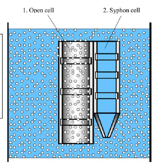
The syphon only allows slurry to enter, whereas the open cylinder allows both slurry and bubbles to pass through. Both the syphon and open chamber are equipped with three electrodes along their length to measure the conductivity of the medium within them. The gas hold-up is then calculated by the following formula:
$\varepsilon_g=\frac{1-\frac{\kappa_{slg}}{\kappa{sl}}}{1+0.5\frac{\kappa_{slg}}{\kappa{sl}}}$
Superficial gas velocity, Jg
The superficial gas velocity, also known as ‘gas rate’, is a measure of the linear velocity of the gas rising upwards through the pulp phase. It is defined as the volume of gas crossing a unit cross section area (e.g. of the flotation cell) per unit time as follows:
$J_g = \frac{\nu_{air}}{A_{cell}}$
In units of length/time, where νair is the volumetric flow rate of air (or gas) and Acell is the cross sectional area of the flotation cell. The superficial gas velocity measured in most flotation cells ranges between 0.5 and 2.8 cm/s, with tank cells in the range of 0.7 to 1.4 cm/s, 1.3 to 1.8 cm/s being typical of mechanical cells and the highest numbers found in column cells5. Less than 0.5 cm/s again indicates insufficient air entering the cell, resulting in a decrease in pulp phase recovery. Higher than 2-3 cm/s can cause flooding, or where pulp is recovered as concentrate due to the high turbulence.
Superficial gas velocity can be measured experimentally in a few ways:
- Directly, by using a flow meter on the exit of the tube to measure air rate and dividing by the tube cross-sectional area.
- By measuring the rate of descent of the water in a transparent tube once the exit valve is closed which approximates the air velocity.
- Measuring the rate of increase in pressure once the exit valve is closed. With pressure measured in cm of water, the rate of increase approximates the air velocity.
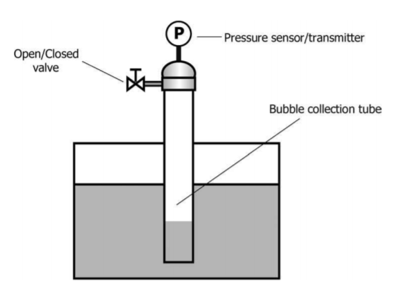
Most Jg probes work on the principle of water displacement over a known distance per unit time, resulting in the gas velocity, however, the measurement can also be calibrated from the volumetric air flowrate distributed to individual cells. Figure 3 shows a probe developed at McGill University which is inserted into the pulp at a given depth and a valve at the top is closed. The pressure increase due to gas build-up within the chamber is then recorded with time. Because this measurement also requires knowledge of the bulk density of the pulp, it is usually taken at two depths to back-out its value as well. The probes also have a means of determining cell pulp level in real-time so as to correct Jg measurements accordingly.
Another probe developed at JKMRC in Brisbane, Australia consists of a Perspex tube with a pinch valve at one end and a water-release-to-atmosphere valve at the other. The probe is shown in Figure 4.

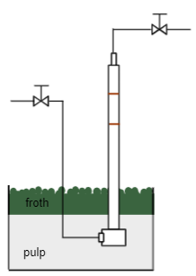
A diagram of the probe is also shown in Figure 5. The pinch valve is first closed, then the tube is inserted vertically into the cell, filled with water from the top and then the water valve is closed. The pinch valve is then opened in order to allow bubbles from the cell to rise into the tube. Air thus accumulates in the tube and displaces water within the same. The time, t, required for air to displace water as well as the length travelled by the water, L, are recorded. The superficial gas velocity is then calculated from these experimental values per:
$J_{g,exp} = \frac{L}{t}$
This experimentally-determined superficial gas velocity is then corrected to obtain a value independent of the measurement conditions per the following:
$J_{g,corr} = J_{g,exp} \frac{P_{atm}+\rho_PgH_P-\rho_WgH_w}{P_{atm}+\rho_PgH_P}$
Where Patm is the atmospheric pressure, 𝜌P is the density of the aerated pulp, HP is the pulp depth from the pulp/froth interface to the bottom of the Jg probe, 𝜌W is the density of aerated water inside the probe, HW is the height from the bottom of the probe to the second mark and g is the gravitational acceleration. The densities, 𝜌P and 𝜌W are, in turn, calculated using the gas hold-up 𝜀g per equations 8 and 9, respectively. In these equations, 𝜌slurry the density of slurry, and 𝜌water is that of pure water.
$\rho_P = \rho_{slurry}(1-\varepsilon_g)$
$\rho_W = \rho_{water}(1-\varepsilon_g)$
Bubble size, db
The bubbles contained within the pulp must be the correct size for particle/bubble interactions to occur. There have been various methods developed to measure the bubble size within the pulp phase, with a trend in recent years towards photographic techniques.
The average bubble size, or arithmetic mean diameter, (d10) can be calculated from measuring a significant number of bubbles and determining the average size. However, research has indicated that the Sauter mean bubble size better represents the bubble size distribution, which is given by the following formula:
$d_{32}=\frac{\sum_{i=1}^{n}d^3_i}{\sum_{i=1}^{n}d^2_i}$
where di is the individual bubble size (i.e. diameter). In general, the average diameter (d10) and Sauter mean diameter are not the same; the wider the range of bubble sizes in a particular distribution, the larger is the Sauter mean diameter compared to the arithmetic mean. The Sauter mean bubble size can be thought of as a weighted sum of bubble diameters in which the weights are terms proportional to the bubble’s surface area, namely, di2. Therefore, d32 can be expressed as (with weight term in bold):
$d_{32}=\frac{\sum_{i=1}^{n}d_i \cdot \mathbf{d^2_i}}{\sum_{i=1}^{n}d^2_i}$
The important point is that the emphasis is on the surface area, in which the Sauter mean bubble size represents the mean size of a bubble population with a given volume/surface area ratio (see Eq. 12). When the volume/surface area ratio is minimal, a given volume of gas dispersed will have maximum surface area under the conditions, a state which is favorable in flotation, in particular for finer particles. In other words, the lower the value of the Sauter mean diameter, the better the dispersion of the gas is in terms of small bubbles. Any non-uniformity in the distribution, say by presence of a small population of large bubbles will skew the Sauter mean diameter to larger values given that these are given more weight.
$d_{32}=\frac{\text{total air volume in the cell}}{\text{total bubble surface area in the cell}}$
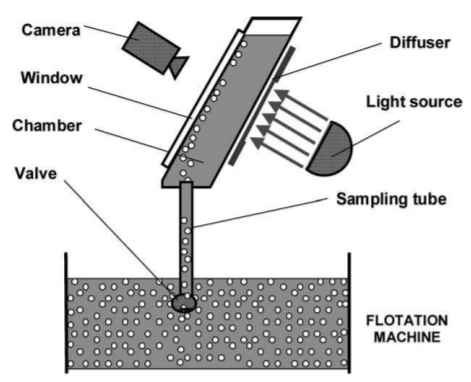
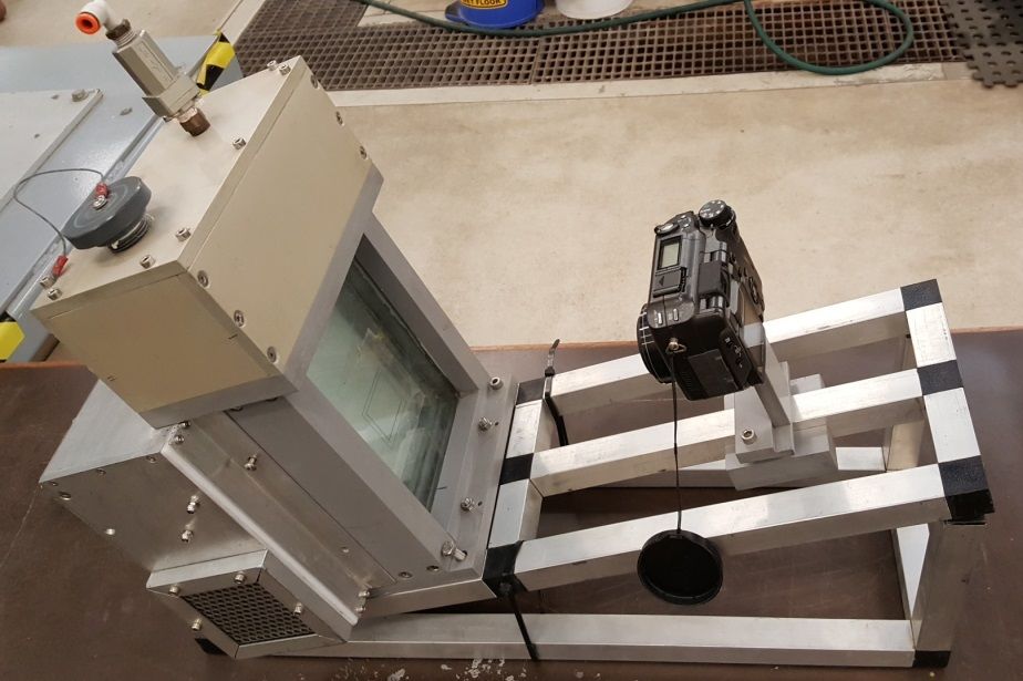
Determination of bubble size distributions in a cell is done through a procedure that includes sampling and imaging of the bubbles followed by image processing for statistical calculations using a bubble size analyzer. As shown in Figure 6, the bubble size analyzer’s chamber is pre-filled with process water (to account for chemical composition of the slurry), its sampling tube is then inserted to a given depth and location within the flotation cell (with the valve closed), the valve is opened and bubbles rise by natural buoyancy through the tube into the chamber where they are imaged through the clear window side with a high-speed, high-resolution camera. Note that the chamber is backlit through a diffuser with a light-source. Images are then analyzed by dedicated software to determine bubble size distributions. Figure 7 shows an example of an actual bubble size analyzer.
Typical measurements in mechanical flotation cells range from 1-1.5 mm, while column cells can contain bubbles as large as 3-5 mm, depending on the sparger mechanism. In general, finer bubbles are more efficient at collecting finer particles, and coarse bubbles are more efficient for coarser particles.
Bubble surface area flux, Sb
The bubble surface area flux combines the measured superficial gas velocity and bubble size values to give an overall indication of the gas dispersion properties within a flotation cell:
$S_b = 6 \cdot \frac{J_g}{d_b}$
The flotation rate constant has been demonstrated to be linearly related to the bubble surface area flux7 as suggested also in equation 1, indicating that higher Sb values will result in higher recoveries across the pulp phase. However, it is noted that there is an optimum level of Sb for flotation cells, and operating at higher values will lead to significant turbulence, causing the particles to drop off the bubbles and ultimately reduce the cell recovery. Typical values of the bubble surface area flux range from 30 – 70 sec for both mechanical and column flotation cells.
Froth recovery
The froth phase is critical in determining the overall cell performance. Even if the pulp phase performs at its optimum levels, if the froth recovery is low, there will be significant drop-back of particles to the pulp phase and a lower overall cell recovery. However, increasing the froth recovery (generally by reducing the froth depth) can also reduce the concentrate grade, due to entrainment of gangue material. There will usually be a balance between grade (deeper froths) and recovery (shallower froths) for each cell or bank, depending on the duty.
Froth recovery can be defined as the efficiency of the froth phase, i.e., the proportion of particles attached to the bubbles entering the froth that are recovered in the concentrate. The measurements range from 0-100%, although most industrial cells have froth recoveries of less than 30%.
Froth recovery can be measured by changing the froth depth and determining the linear relationship between overall recovery and froth depth, or by special sensors and techniques such as the bubble load device and the mass balance technique. Both of these methods are focused on determining the flowrate of particles attached to bubbles entering the froth phase, with the bubble load device measuring this flowrate directly, and the mass balance technique calculating the flowrate from other measurements.
Residence time, 𝛕
Residence time is defined as how long air, liquid or slurry remains in the flotation cell or bank. It can be calculated from:
$\tau=\frac{V_{pulp}(1-\varepsilon_g)}{Q_{tails}}$
where Vpulp is the effective pulp volume (overall cell volume reduced by the volume of the mechanism and volume of the froth), g is the gas hold-up and Qtails is the volumetric flowrate of the tails passing out from the cell or bank.
Residence time can also be measured by introducing a liquid tracer to the cell or bank and collecting samples over known time intervals. The residence time as well as the proportion of perfectly mixed regions within the cell or bank can be determined using a tanks-in-series model.
Increasing residence time increases the time available for bubble/particle interactions to occur and will generally result in higher recoveries, however, often at the expense of grade. Residence time can be increased by either installing more flotation cells (requiring capital expenditure) or by reducing the tonnage through the circuit. It should be noted that higher residence time is not always the best for optimum metallurgical performance.
Entrainment and water recovery
Entrainment is the mechanism by which non-floating material is recovered in the concentrate. This material is dragged next to and behind the rising bubbles into the froth phase, where it can either continue to rise upwards with the bubbles, or drain back to the pulp phase. Entrainment is non-selective in that it affects all minerals equally, depending on the physical properties such as density and size, rather than surface characteristics.
Recovering entrained species will often be detrimental to the concentrate grade, and many methods have been tried to reduce the amount of material recovered by entrainment. As entrainment is directly related to the recovery of water across the cell or bank, reducing the water recovery will reduce the recovery by entrainment. However, practically there are limitations to lowering the water recovery and maintaining a stable froth phase. Wash water is an effective method for reducing the water recovery from the pulp to the froth phase, and this also assists in washing the entrained particles back to the pulp phase.
Entrainment is generally measured by a tracer, usually already present in the ore. Tracking the recovery of a non-floating, liberated mineral to the concentrates within the circuit gives an indication of the recovery by entrainment. If there is no suitable mineral naturally present, mineralogical analysis such as MLA can be used.
Summary
Measuring the various properties and sub-processes of the feed stream, the pulp zone and the froth zone in flotation cells at the plant level is the first step to understanding the behaviour of particles within the system. Once a baseline measurement has been conducted, issues or deficiencies are diagnosed and opportunities for potential improvement can be identified and implemented to achieve the optimum metallurgical performance.
There are several approaches to achieve this optimization; the one described above is from University of Queensland – JKTech Pty Limited.
References
- Ahmed N., Jameson G.J. Flotation kinetics. Mineral Procesing and Extractive Metallurgy Review. 1989 Feb 2; 5(1-4):77-99.
- Alexander, D.J., Morrison, R.D. Rapid estimation of floatability components in industrial flotation plants. Minerals Engineering 1998, 11:133-143.
- Dahlke, R., Gomez, C., Finch, J.A. Operating range of a flotation cell determined from gas holdup vs. gas rate. Minerals Engineering. 2005 Aug 1; 18(9):977-80.
- Deglon D.A., Sawyerr F., O'Connor C.T. A model to relate the flotation rate constant and the bubble surface area flux in mechanical flotation cells. Minerals Engineering. 1999 Jun 1;12(6):599-608.
- Deglon D.A., Egya-Mensah D., Franzidis J.P. Review of hydrodynamics and gas dispersion in flotation cells on South African platinum concentrators. Minerals Engineering. 2000 Mar 1;13(3):235-44.
- Goh, S.W., Buckley, A.N., Lamb, R.N., Woods, R. The ability of static secondary ion mass spectrometry to discriminate submonolayer from multilayer adsorption of thiol collectors. Minerals Engineering 2006, 19:571-581.
- Gorain, B.K., Franzidis, J.P., Manlapig, E.V. Studies on impeller type, impeller speed and air flow rate in an industrial scale flotation cell. Part 4: Effect of bubble surface area flux on flotation performance. Minerals Engineering. 1997 Apr 1; 10(4):367-79.
- Harris, M.C. A practical framework for flotation circuit modelling and simulation. Paper presented at SAIChE ’97, the 8th National Meeting of the South African Institute of Chemical Engineers, Cape Town, 16-18 April 1997.
- Hernandez, H., Gomez, C.O., Finch JA. Gas dispersion and de-inking in a flotation column. Minerals Engineering. 2003 Aug 1; 16(8):739-44.
- Nesset, J.E., Hernandez-Aguilar, J.R., Acuna, C., Gomez, C.O., Finch, J.A. Some gas dispersion characteristics of mechanical flotation machines. Minerals Engineering. 2006 May 1; 19(6-8):807-15.
- Wills, B.A., Finch J. Wills' mineral processing technology: an introduction to the practical aspects of ore treatment and mineral recovery. Butterworth-Heinemann; 2015 Sep 1.
- Woods, R. Electrochemistry of Sulfide Flotation: Flotation. AIME, New York. 1976:298.
- Woods, R. Electrochemical potential controlling flotation. International Journal of Mineral Processing 2003, 72:151-162.